1 Introduction
The fractional calculus (e.g. Kilbas et al., 2006; Podlubny, 1999; Rubin, 1996) is treated as a branch of mathematical analysis dealing with differential-integral equations, in which the integrals are of the convolutional type and have power-type kernels. The fractional calculus refers to the fractional integration and fractional differentiation. It can be seen in the extensive literature in the past few decades that the fractional calculus has received increasing attention for its applications in science and engineering – it is difficult to list examples of literature without omitting even the most important ones. This work mainly deals with the development and investigation of numerical methods for the fractional integrals.
We recall the following definitions of the Riemann–Liouville fractional integrals. The left-sided fractional integral of order $\alpha \gt 0$ of the given function $y(x)$ on the interval $[a,b]$ is defined as follows (Kilbas et al., 2006; de Oliveira and Machado, 2014)
where Γ denotes the Gamma function. Whereas, the right-sided fractional integral is of the form
The Riesz fractional integral (known also as the Riesz potential), in general, is defined in the infinite n-dimensional domain (Rubin, 1996; Kilbas et al., 2006). Here, we limit our considerations to its one-dimensional definition in the finite interval of the real axis, and then it can be regarded as the linear combination of the left- and right-sided Riemann–Liouville integrals. The Riesz fractional integral of order $\alpha \gt 0$, $\alpha \ne 1,3,5,\dots $ of the function $y(x)$ on the finite interval $[a,b]$ is defined as (see: Kilbas et al., 2006)
(1)
\[ {I_{{a^{+}}}^{\alpha }}y(x)=\frac{1}{\Gamma (\alpha )}{\int _{a}^{x}}\frac{y(\xi )}{{(x-\xi )^{1-\alpha }}}d\xi ,\hspace{1em}\text{for}\hspace{2.5pt}x\gt a,\](2)
\[ {I_{{b^{-}}}^{\alpha }}y(x)=\frac{1}{\Gamma (\alpha )}{\int _{x}^{b}}\frac{y(\xi )}{{(\xi -x)^{1-\alpha }}}d\xi ,\hspace{1em}\text{for}\hspace{2.5pt}x\lt b.\](3)
\[\begin{aligned}{}{^{R}}{I_{[a,b]}^{\alpha }}y(x)& =\frac{1}{2\Gamma (\alpha )\cos (\alpha \pi /2)}{\int _{a}^{b}}\frac{y(\xi )}{{|\xi -x|^{1-\alpha }}}d\xi \\ {} & =\frac{1}{2\cos (\alpha \pi /2)}\big({I_{{a^{+}}}^{\alpha }}y(x)+{I_{{b^{-}}}^{\alpha }}y(x)\big),\hspace{1em}\text{for}\hspace{2.5pt}a\lt x\lt b.\end{aligned}\]The above fractional integral operators play an important role in the fractional calculus, especially to transform fractional differential equations into fractional integral equations. Therefore, among others, it is necessary to develop appropriate numerical methods for approximate evaluation of these fractional integrals. In view of the numerous applications of the fractional integral operators, there is great demand for efficient and accurate algorithms for their numerical calculations, especially for the integrand functions that have complicated forms or the explicit analytical forms of the fractional integrals that are so far unknown. Generally, different ways of discretization of the integrand function yield a series of quadrature formulas, whereas different formulas of coefficients in these quadratures give different accuracies. Numerical approximations of the fractional integrals are most often based on polynomial interpolation from which numerical schemes can be derived with a specified accuracy. Among the pioneering works in this field, the book by Oldham and Spanier (1974) can be distinguished. The reviews of different numerical methods (so far known) for fractional integrals and derivatives can be found in Cai and Li (2020), Li and Zeng (2015), Almeida et al. (2015), Blaszczyk and Siedlecki (2014), Baleanu et al. (2012), Malinowska et al. (2015), Blaszczyk et al. (2018), Odibat (2006), Dimitrov (2021), Budak et al. (2023). Due to the wide applications of fractional calculus, it is becoming increasingly important to develop numerical algorithms with high accuracy, fast convergence and less storage memory.
In this work, we focused primarily on the study of numerical algorithms for approximation of fractional integrals (1)–(3) by applying several interpolation methods for the integrand function using different kinds of splines. Next, we derived and presented general numerical integration schemes for the left and right-sided Riemann–Liouville and the Riesz fractional integrals. For each numerical scheme, we estimated the computational error using analytical methods. We tested the quality of the obtained numerical algorithms on three examples by examining numerical errors and determining the experimental order of convergence.
2 Numerical Algorithms
The integrand function $y(x)$ given in Eqs. (1)–(3) should be defined on interval $[a,b]$ and sufficiently smooth. In the proposed approach, function $y(x)$ is replaced by same interpolation formulas, e.g. an interpolation polynomial of arbitrary degree or an interpolation spline, as
Often instead of using high-degree polynomials, one can apply the spline curves (Press et al., 2007; Engeln-Müllges and Uhlig, 1996). The advantage of such an approach is that the spline curves are at most third degree polynomials and hence the oscillations between interpolation points are characterized by smaller amplitude and, after all, the splines are only piecewise continuous.
2.1 Spline Interpolations
The spline is a set of piecewise polynomials linked in the set of points. Let us assume that the interval $[a,b]$ is divided into N sub-intervals $[{x_{i}},{x_{i+1}}]$, for $i=0,1,\dots ,N-1$, with the constant step length $\Delta x=(b-a)/N$. The coordinates of $N+1$ nodal points are the following: $a={x_{0}}\lt {x_{1}}\lt \cdots \lt {x_{N}}=b$, ${x_{i}}=a+i\hspace{0.1667em}\Delta x$. At the given set of points, the values of function $y(x)$ are determined as ${y_{i}}=y({x_{i}})$, for $i=0,1,\dots ,N$. The piecewise function $s(x)$ can be expressed as
where ${s_{i}}(x)$ are polynomials of degree p in each sub-interval $[{x_{i}},{x_{i+1}}]$, for $i=0,1,\dots ,N-1$, and here we write these polynomials in the form
where ${c_{k,i}}$, for $k=0,1,\dots ,p$, are the coefficients of polynomial ${s_{i}}(x)$ in i-th sub-interval $[{x_{i}},{x_{i+1}}]$. The way of determination of these coefficients depends on the kind of spline interpolation used. Additionally, the important feature of the spline $s(x)$ that interpolates the set of the data points $({x_{0}},{y_{0}}),({x_{1}},{y_{1}}),\dots ,({x_{N}},{y_{N}})$ is the relationship $s({x_{i}})={y_{i}}$, for $i=0,1,\dots ,N$.
(5)
\[ s(x)=\left\{\begin{array}{l@{\hskip4.0pt}l}{s_{0}}(x),\hspace{1em}& \text{if}\hspace{2.5pt}x\in [{x_{0}},{x_{1}}],\\ {} {s_{1}}(x),\hspace{1em}& \text{if}\hspace{2.5pt}x\in [{x_{1}},{x_{2}}],\\ {} \dots \hspace{1em}\\ {} {s_{N-1}}(x),\hspace{1em}& \text{if}\hspace{2.5pt}x\in [{x_{N-1}},{x_{N}}],\end{array}\right.\]2.1.1 Linear Spline Interpolation
The linear interpolation is the simplest form of interpolation where the set of the data points is approximated by a piecewise linear function (the first degree polynomial), which means that the adjacent data points $({x_{i}},{y_{i}})$ and $({x_{i+1}},{y_{i+1}})$, for $i=0,1,\dots ,N-1$, wherein $N\geqslant 2$, are connected by straight lines. The polynomial of first degree ($p=1$) in i-th sub-interval is constructed as
The linear Lagrange interpolating polynomial in the interval $x\in [{x_{i}},{x_{i+1}}]$, for $i=0,1,\dots ,N-1$, that passes through the points $({x_{i}},{y_{i}})$ and $({x_{i+1}},{y_{i+1}})$ results from the relation
and hence, the polynomial coefficients in Eq. (7) are as follows
Moreover, the error term in i-th interval is given as
where ${\bar{x}_{i}}\in [{x_{i}},{x_{i+1}}]$ is a certain point in the interval. The error term involves ${y^{\prime\prime }}$, so the linear spline gives the exact result for any function $y(x)$, where the second derivative is equal to zero. In literature, this approach used for integration is known as the trapezoidal rule (Press et al., 2007).
(8)
\[\begin{aligned}{}y(x)& =\frac{x-{x_{i+1}}}{{x_{i}}-{x_{i+1}}}y({x_{i}})+\frac{x-{x_{i}}}{{x_{i+1}}-{x_{i}}}y({x_{i+1}})+\frac{{y^{\prime\prime }}({\bar{x}_{i}})}{2!}(x-{x_{i}})(x-{x_{i+1}})\\ {} & ={y_{i}}+\frac{{y_{i+1}}-{y_{i}}}{\Delta x}(x-{x_{i}})+\frac{{y^{\prime\prime }}({\bar{x}_{i}})}{2}(x-{x_{i}})(x-{x_{i+1}})\\ {} & ={s_{i}}(x)+\textit{Err}{1_{i}}(x),\end{aligned}\](10)
\[ \textit{Err}{1_{i}}(x)=\frac{{y^{\prime\prime }}({\bar{x}_{i}})}{2}(x-{x_{i}})(x-{x_{i+1}}),\]2.1.2 Quadratic Spline Interpolation
In this kind of approximation, the second degree polynomial ($p=2$) in each i-th sub-interval is used
where $x\in [{x_{i}},{x_{i+1}}]$, for $i=0,1,\dots ,N-1$, and $N\geqslant 2$ must also be even. To determine the coefficients of parabola (quadratic segment), three data points are needed, and hence each parabola spans two sub-intervals.
Here, we suppose that function $y(x)$ in the considered double interval $[{x_{i-1}},{x_{i+1}}]$, for $i=1,3,\dots ,N-1$, is expanded in the Taylor polynomial of third order about the central point ${x_{i}}$ as
where ${\bar{x}_{1i}}\in [{x_{i-1}},{x_{i+1}}]$ is a certain point in the interval. The values of ${y^{\prime }}({x_{i}})$ and ${y^{\prime\prime }}({x_{i}})$ in Eq. (12) are replaced by well-known relationships
where ${\bar{x}_{2i}}\in [{x_{i-1}},{x_{i+1}}]$ and ${\bar{x}_{3i}}\in [{x_{i-1}},{x_{i+1}}]$, and hence it was obtained
or written in the form
where
and
wherein ${\bar{x}_{i}}\in [{x_{i-1}},{x_{i+1}}]$ is taking into account as common values of ${x_{i}}$, ${\bar{x}_{1i}}$, ${\bar{x}_{2i}}$ and ${\bar{x}_{3i}}$.
(12)
\[\begin{aligned}{}y(x)& =y({x_{i}})+{y^{\prime }}({x_{i}})(x-{x_{i}})+\frac{{y^{\prime\prime }}({x_{i}})}{2!}{(x-{x_{i}})^{2}}+\frac{{y^{\prime\prime\prime }}({x_{i}})}{3!}{(x-{x_{i}})^{3}}\\ {} & \hspace{1em}+\frac{{y^{(4)}}({\bar{x}_{1i}})}{4!}{(x-{x_{i}})^{4}},\end{aligned}\](13)
\[ \begin{aligned}{}& {y^{\prime }}({x_{i}})=\frac{1}{2\Delta x}\big(y({x_{i+1}})-y({x_{i-1}})\big)-\frac{{(\Delta x)^{2}}}{6}{y^{\prime\prime\prime }}({\bar{x}_{2i}}),\\ {} & {y^{\prime\prime }}({x_{i}})=\frac{1}{{(\Delta x)^{2}}}\big(y({x_{i+1}})-2y({x_{i}})+y({x_{i-1}})\big)-\frac{{(\Delta x)^{2}}}{12}{y^{(4)}}({\bar{x}_{3i}}),\end{aligned}\](14)
\[\begin{aligned}{}y(x)& =y({x_{i}})+\bigg(\frac{y({x_{i+1}})-y({x_{i-1}})}{2\Delta x}-\frac{{(\Delta x)^{2}}}{6}{y^{\prime\prime\prime }}({\bar{x}_{2i}})\bigg)(x-{x_{i}})\\ {} & \hspace{1em}+\frac{1}{2!}\bigg(\frac{y({x_{i+1}})-2y({x_{i}})+y({x_{i-1}})}{{(\Delta x)^{2}}}-\frac{{(\Delta x)^{2}}}{12}{y^{(4)}}({\bar{x}_{3i}})\bigg){(x-{x_{i}})^{2}}\\ {} & \hspace{1em}+\frac{{y^{\prime\prime\prime }}({x_{i}})}{3!}{(x-{x_{i}})^{3}}+\frac{{y^{(4)}}({\bar{x}_{1i}})}{4!}{(x-{x_{i}})^{4}},\end{aligned}\](15)
\[ y(x)={s_{i}}(x)+\textit{Err}{2_{i}}(x),\hspace{1em}\text{for}\hspace{2.5pt}x\in [{x_{i-1}},{x_{i+1}}],\](16)
\[ {s_{i}}(x)={y_{i}}+\frac{{y_{i+1}}-{y_{i-1}}}{2\Delta x}(x-{x_{i}})+\frac{{y_{i+1}}-2{y_{i}}+{y_{i-1}}}{2{(\Delta x)^{2}}}{(x-{x_{i}})^{2}}\](17)
\[\begin{aligned}{}\textit{Err}{2_{i}}(x)& =\frac{1}{6}{y^{\prime\prime\prime }}({x_{i}}){(x-{x_{i}})^{3}}-\frac{{(\Delta x)^{2}}}{6}{y^{\prime\prime\prime }}({\bar{x}_{2i}})(x-{x_{i}})\\ {} & \hspace{1em}+\frac{1}{24}{y^{(4)}}({\bar{x}_{1i}}){(x-{x_{i}})^{4}}-\frac{{(\Delta x)^{2}}}{24}{y^{(4)}}({\bar{x}_{3i}}){(x-{x_{i}})^{2}}\\ {} & \cong \frac{1}{6}\big({(x-{x_{i}})^{3}}-{(\Delta x)^{2}}(x-{x_{i}})\big){y^{\prime\prime\prime }}({\bar{x}_{i}})\\ {} & \hspace{1em}+\frac{1}{24}\big({(x-{x_{i}})^{4}}-{(\Delta x)^{2}}{(x-{x_{i}})^{2}}\big){y^{(4)}}({\bar{x}_{i}}),\end{aligned}\]In order to maintain a uniform form of the spline notation (as in Eq. (11)), two cases are considered
If i is odd (i.e. $i=1,3,\dots ,N-1$), then the coefficients ${\bar{c}_{k,i}}$ can be taken directly from Eq. (16) as
and then the relationships ${s_{i}}({x_{i-1}})={y_{i-1}}$, ${s_{i}}({x_{i}})={y_{i}}$, ${s_{i}}({x_{i+1}})={y_{i+1}}$ occur.
(19)
\[ {\bar{c}_{0,i}}={y_{i}},\hspace{2em}{\bar{c}_{1,i}}=\frac{{y_{i+1}}-{y_{i-1}}}{2\Delta x},\hspace{2em}{\bar{c}_{2,i}}=\frac{{y_{i-1}}-2{y_{i}}+{y_{i+1}}}{2{(\Delta x)^{2}}},\]If i is even (i.e. $i=0,2,\dots ,N-2$), then the coefficients ${\bar{\bar{c}}_{k,i}}$ are calculated from the transformation of Eq. (16) by substitution $i\gets i+1$ on the right side of equation, and hence they have the following forms
and the properties ${s_{i}}({x_{i}})={y_{i}}$, ${s_{i}}({x_{i+1}})={y_{i+1}}$, ${s_{i}}({x_{i+2}})={y_{i+2}}$ hold.
(20)
\[ {\bar{\bar{c}}_{0,i}}={y_{i}},\hspace{2em}{\bar{\bar{c}}_{1,i}}=\frac{-3{y_{i}}+4{y_{i+1}}-{y_{i+2}}}{2\Delta x},\hspace{2em}{\bar{\bar{c}}_{2,i}}=\frac{{y_{i}}-2{y_{i+1}}+{y_{i+2}}}{2{(\Delta x)^{2}}},\]As can be seen in the first case, the quadratic segment is defined in the interval $[{x_{i}},{x_{i+2}}]$ (for i even), while in the second case it is defined in the interval $[{x_{i-1}},{x_{i+1}}]$ (for i odd), but in fact, both quadratic segments are identical in two adjacent sub-intervals. This approach will simplify the notations of numerical integration later in the work.
2.1.3 Cubic Spline Interpolation
The cubic splines produce a curve that appears to be seamless and has smooth characteristics. A piecewise continuous curve passes through each of the data points $({x_{i}},{y_{i}})$, for $i=0,1,\dots ,N$, wherein $N\geqslant 4$, in the given order and the separate polynomial of third degree ($p=3$) (so-called the cubic polynomial segment) in each sub-interval has its own set of coefficients, i.e.
where $x\in [{x_{i}},{x_{i+1}}]$, for $i=0,1,\dots ,N-1$. These four coefficients ${c_{0,i}}$, ${c_{1,i}}$, ${c_{2,i}}$ and ${c_{3,i}}$ for i-th polynomial, in each of the N sub-intervals should be determined, and hence, in order to define the whole spline, a total of $4N$ independent dependencies imposed on the spline are required.
(21)
\[ {s_{i}}(x)={c_{0,i}}+{c_{1,i}}(x-{x_{i}})+{c_{2,i}}{(x-{x_{i}})^{2}}+{c_{3,i}}{(x-{x_{i}})^{3}},\]In the case of this kind of spline, the following assumptions are made (Burden et al., 2016):
-
– the polynomials match the data points at both ends of each i-th sub-interval: ${s_{i}}({x_{i}})={y_{i}}$, ${s_{i}}({x_{i+1}})={y_{i+1}}$, for $i=0,1,\dots ,N-1$, (two conditions for each sub-interval give $2N$ dependencies in total).
-
– the spline interpolation must be smooth, therefore the following requirements are assumed for the first and second derivatives of the spline (which means that the slope and the curvature must be equal for each pair of neighbouring polynomials that join at each data point): ${s^{\prime }_{i-1}}({x_{i}})={s^{\prime }_{i}}({x_{i}})$, ${s^{\prime\prime }_{i-1}}({x_{i}})={s^{\prime\prime }_{i}}({x_{i}})$, for $i=1,2,\dots ,N-1$, (two conditions for each internal node give further $2N-2$ dependencies).
-
– the missing two additional conditions should be determined on the basis of the assumed integer order derivatives of the function $y(x$) in the boundary nodes ${x_{0}}$ and ${x_{N}}$ (colloquially called the end point conditions). Three variants of the cubic spline constructions are considered:where ${Y^{\prime }_{0}}$, ${Y^{\prime\prime }_{0}}$, ${Y^{\prime\prime\prime }_{0}}$, ${Y^{\prime }_{N}}$, ${Y^{\prime\prime }_{N}}$ and ${Y^{\prime\prime\prime }_{N}}$ correspond to the values of the first, second and third order derivatives of the function $y(x)$ at the nodes ${x_{0}}$ and ${x_{N}}$, respectively. In principle, any combination of derivative orders at both boundary nodes can be considered (e.g. ${s^{\prime\prime\prime }_{0}}({x_{0}})$ and ${s^{\prime }_{N-1}}({x_{N}})$).
-
• variant 1: ${s^{\prime }_{0}}({x_{0}})={Y^{\prime }_{0}}$, ${s^{\prime }_{N-1}}({x_{N}})={Y^{\prime }_{N}}$,
-
• variant 2: ${s^{\prime\prime }_{0}}({x_{0}})={Y^{\prime\prime }_{0}}$, ${s^{\prime\prime }_{N-1}}({x_{N}})={Y^{\prime\prime }_{N}}$,
-
• variant 3: ${s^{\prime\prime\prime }_{0}}({x_{0}})={Y^{\prime\prime\prime }_{0}}$, ${s^{\prime\prime\prime }_{N-1}}({x_{N}})={Y^{\prime\prime\prime }_{N}}$,
-
To determine the coefficients in Eq. (21), we used substitutions (see: Burden et al., 2016) in order to reduce the number of coefficients to be determined
and hence, the cubic spline in the i-th sub-interval (Eq. (21)) can be written in the form
(22)
\[\begin{aligned}{}& {c_{0,i}}={y_{i}},\\ {} & {c_{1,i}}=\frac{{y_{i+1}}-{y_{i}}}{\Delta x}-\frac{\Delta x}{3}({c_{2,i+1}}+2{c_{2,i}}),\\ {} & {c_{3,i}}=\frac{1}{3\Delta x}({c_{2,i+1}}-{c_{2,i}}),\end{aligned}\]It can now be seen that only $N+1$ unknown coefficients ${c_{2,i}}$ need to be determined (the last one with the index N is used to evaluate ${c_{1,N-1}}$ and ${c_{3,N-1}}$). The first, second and third derivatives of the spline ${s_{i}}(x)$ are as follows
(24)
\[ \begin{aligned}{}& {s^{\prime }_{i}}(x)=\bigg(\frac{{y_{i+1}}-{y_{i}}}{\Delta x}-\frac{\Delta x}{3}({c_{2,i+1}}+2{c_{2,i}})\bigg)+2{c_{2,i}}(x-{x_{i}})\\ {} & \phantom{{s^{\prime }_{i}}(x)=}+\frac{1}{\Delta x}({c_{2,i+1}}-{c_{2,i}}){(x-{x_{i}})^{2}},\\ {} & {s^{\prime\prime }_{i}}(x)=2{c_{2,i}}+\frac{2}{\Delta x}({c_{2,i+1}}-{c_{2,i}})(x-{x_{i}}),\\ {} & {s^{\prime\prime\prime }_{i}}(x)=\frac{2}{\Delta x}({c_{2,i+1}}-{c_{2,i}}).\end{aligned}\]It is easy to check that the conditions: ${s_{i}}({x_{i}})={y_{i}}$, ${s_{i}}({x_{i+1}})={y_{i+1}}$, for $i=0,1,\dots ,N-1$, and ${s^{\prime\prime }_{i-1}}({x_{i}})={s^{\prime\prime }_{i}}({x_{i}})$, for $i=1,2,\dots ,N-1$, are always present. While, from the conditions ${s^{\prime }_{i-1}}({x_{i}})={s^{\prime }_{i}}({x_{i}})$, for $i=1,2,\dots ,N-1$, as a result, the following dependencies are obtained
To complete the system of $N+1$ linear equations, two dependencies resulting from the end point conditions should be added. If the points ${x_{0}}$ and ${x_{N}}$ are inserted into the appropriate spline derivatives, then we get
(26)
\[ \begin{aligned}{}& {s^{\prime }_{0}}({x_{0}})=\frac{{y_{1}}-{y_{0}}}{\Delta x}-\frac{\Delta x}{3}({c_{2,1}}+2{c_{2,0}}),\\ {} & {s^{\prime\prime }_{0}}({x_{0}})=2{c_{2,0}},\\ {} & {s^{\prime\prime\prime }_{0}}({x_{0}})=\frac{2}{\Delta x}({c_{2,1}}-{c_{2,0}}),\\ {} & {s^{\prime }_{N-1}}({x_{N}})=\frac{{y_{N}}-{y_{N-1}}}{\Delta x}+\frac{\Delta x}{3}({c_{2,N-1}}+2{c_{2,N}}),\\ {} & {s^{\prime\prime }_{N-1}}({x_{N}})=2{c_{2,N}},\\ {} & {s^{\prime\prime\prime }_{N-1}}({x_{N}})=\frac{2}{\Delta x}({c_{2,N}}-{c_{2,N-1}}).\end{aligned}\]Hence, depending on the assumed variant of the cubic spline construction, the missing end point conditions can be determined in the forms
-
• variant 1: $2{c_{2,0}}+{c_{2,1}}=3\bigg(\displaystyle\frac{{y_{1}}-{y_{0}}}{{(\Delta x)^{2}}}-\displaystyle\frac{{{Y^{\prime }}_{0}}}{\Delta x}\bigg)$,${c_{2,N-1}}+2{c_{2,N}}=3\bigg(\displaystyle\frac{{{Y^{\prime }}_{N}}}{\Delta x}-\displaystyle\frac{{y_{N}}-{y_{N-1}}}{{(\Delta x)^{2}}}\bigg)$,
-
• variant 2: ${c_{2,0}}=\displaystyle\frac{1}{2}{Y^{\prime\prime }_{0}}$, ${c_{2,N}}=\displaystyle\frac{1}{2}{Y^{\prime\prime }_{N}}$,
-
• variant 3: ${c_{2,0}}-{c_{2,1}}=-\displaystyle\frac{\Delta x}{2}{Y^{\prime\prime\prime }_{0}}$, $-{c_{2,N-1}}+{c_{2,N}}=\displaystyle\frac{\Delta x}{2}{Y^{\prime\prime\prime }_{N}}$.
The above derived relationships create the linear system of equations that can be written in matrix form
where
and
(27)
\[ \left[\begin{array}{c@{\hskip4.0pt}c@{\hskip4.0pt}c@{\hskip4.0pt}c@{\hskip4.0pt}c@{\hskip4.0pt}c@{\hskip4.0pt}c@{\hskip4.0pt}c}{\gamma _{0,0}}\hspace{1em}& {\gamma _{0,1}}\hspace{1em}& 0\hspace{1em}& 0\hspace{1em}& \cdots \hspace{1em}& 0\hspace{1em}& 0\hspace{1em}& 0\\ {} 1\hspace{1em}& 4\hspace{1em}& 1\hspace{1em}& 0\hspace{1em}& \hspace{1em}& 0\hspace{1em}& 0\hspace{1em}& 0\\ {} 0\hspace{1em}& 1\hspace{1em}& 4\hspace{1em}& 1\hspace{1em}& \hspace{1em}& 0\hspace{1em}& 0\hspace{1em}& 0\\ {} 0\hspace{1em}& 0\hspace{1em}& 1\hspace{1em}& 4\hspace{1em}& \hspace{1em}& 0\hspace{1em}& 0\hspace{1em}& 0\\ {} \vdots \hspace{1em}& \hspace{1em}& \hspace{1em}& \hspace{1em}& \ddots \hspace{1em}& \hspace{1em}& \hspace{1em}& \vdots \\ {} 0\hspace{1em}& 0\hspace{1em}& 0\hspace{1em}& 0\hspace{1em}& \hspace{1em}& 4\hspace{1em}& 1\hspace{1em}& 0\\ {} 0\hspace{1em}& 0\hspace{1em}& 0\hspace{1em}& 0\hspace{1em}& \hspace{1em}& 1\hspace{1em}& 4\hspace{1em}& 1\\ {} 0\hspace{1em}& 0\hspace{1em}& 0\hspace{1em}& 0\hspace{1em}& \cdots \hspace{1em}& 0\hspace{1em}& {\gamma _{N,N-1}}\hspace{1em}& {\gamma _{N,N}}\end{array}\right]\cdot \left[\begin{array}{c}{c_{2,0}}\\ {} {c_{2,1}}\\ {} {c_{2,2}}\\ {} {c_{2,3}}\\ {} \vdots \\ {} {c_{2,N-2}}\\ {} {c_{2,N-1}}\\ {} {c_{2,N}}\end{array}\right]=\left[\begin{array}{c}{d_{0}}\\ {} {d_{1}}\\ {} {d_{2}}\\ {} {d_{3}}\\ {} \vdots \\ {} {d_{N-2}}\\ {} {d_{N-1}}\\ {} {d_{N}}\end{array}\right],\]-
• for variant 1: ${\gamma _{0,0}}=2$, ${\gamma _{0,1}}=1$, ${d_{0}}=3\bigg(\displaystyle\frac{{y_{1}}-{y_{0}}}{{(\Delta x)^{2}}}-\displaystyle\frac{{Y^{\prime }_{0}}}{\Delta x}\bigg)$,${\gamma _{N,N-1}}=1$, ${\gamma _{N,N}}=2$, ${d_{N}}=3\bigg(\displaystyle\frac{{Y^{\prime }_{N}}}{\Delta x}-\displaystyle\frac{{y_{N}}-{y_{N-1}}}{{(\Delta x)^{2}}}\bigg)$,
-
• for variant 2: ${\gamma _{0,0}}=1$, ${\gamma _{0,1}}=0$, ${d_{0}}=\displaystyle\frac{1}{2}{Y^{\prime\prime }_{0}}$,${\gamma _{N,N-1}}=0$, ${\gamma _{N,N}}=1$, ${d_{N}}=\displaystyle\frac{1}{2}{Y^{\prime\prime }_{N}}$,
-
• for variant 3: ${\gamma _{0,0}}=1$, ${\gamma _{0,1}}=-1$, ${d_{0}}=-\displaystyle\frac{\Delta x}{2}{Y^{\prime\prime\prime }_{0}}$,${\gamma _{N,N-1}}=-1$, ${\gamma _{N,N}}=1$, ${d_{N}}=\displaystyle\frac{\Delta x}{2}{Y^{\prime\prime\prime }_{N}}$.
The values of ${Y^{\prime }_{0}}$, ${Y^{\prime\prime }_{0}}$, ${Y^{\prime\prime\prime }_{0}}$, ${Y^{\prime }_{N}}$, ${Y^{\prime\prime }_{N}}$ and ${Y^{\prime\prime\prime }_{N}}$ can be determined directly if the first, second and third order derivatives of function $y(x)$ can be derived analytically, i.e. ${Y^{\prime }_{0}}={y^{\prime }}({x_{0}})$, ${Y^{\prime }_{N}}={y^{\prime }}({x_{N}})$ and so on. Otherwise, we propose to determine the numerical values for them using the forward/backward finite difference schemes of fourth order accuracy (with the uniform grid spacing) in the forms (Fornberg, 1988)
(29)
\[\begin{aligned}{}& \begin{aligned}{}& {Y^{\prime }_{0}}\cong \frac{1}{\Delta x}\bigg(-\frac{25}{12}{y_{0}}+4{y_{1}}-3{y_{2}}+\frac{4}{3}{y_{3}}-\frac{1}{4}{y_{4}}\bigg),\\ {} & {Y^{\prime }_{N}}\cong \frac{1}{\Delta x}\bigg(\frac{25}{12}{y_{N}}-4{y_{N-1}}+3{y_{N-2}}-\frac{4}{3}{y_{N-3}}+\frac{1}{4}{y_{N-4}}\bigg),\end{aligned}\end{aligned}\](30)
\[\begin{aligned}{}& \begin{aligned}{}& {Y^{\prime\prime }_{0}}\cong \frac{1}{{(\Delta x)^{2}}}\bigg(\frac{15}{4}{y_{0}}-\frac{77}{6}{y_{1}}+\frac{107}{6}{y_{2}}-13{y_{3}}+\frac{61}{12}{y_{4}}-\frac{5}{6}{y_{5}}\bigg),\\ {} & {Y^{\prime\prime }_{N}}\cong \frac{1}{{(\Delta x)^{2}}}\bigg(\frac{15}{4}{y_{N}}-\frac{77}{6}{y_{N-1}}+\frac{107}{6}{y_{N-2}}-13{y_{N-3}}+\frac{61}{12}{y_{N-4}}-\frac{5}{6}{y_{N-5}}\bigg),\end{aligned}\end{aligned}\](31)
\[\begin{aligned}{}& \begin{aligned}{}& {Y^{\prime\prime\prime }_{0}}\cong \frac{1}{{(\Delta x)^{3}}}\bigg(-\frac{49}{8}{y_{0}}+29{y_{1}}-\frac{461}{8}{y_{2}}+62{y_{3}}-\frac{307}{8}{y_{4}}+13{y_{5}}-\frac{15}{8}{y_{6}}\bigg),\\ {} & {Y^{\prime\prime\prime }_{N}}\cong \frac{1}{{(\Delta x)^{3}}}\bigg(\frac{49}{8}{y_{N}}-29{y_{N-1}}+\frac{461}{8}{y_{N-2}}-62{y_{N-3}}+\frac{307}{8}{y_{N-4}}\\ {} & \phantom{{Y^{\prime\prime\prime }_{N}}\cong }-13{y_{N-5}}+\frac{15}{8}{y_{N-6}}\bigg).\end{aligned}\end{aligned}\]By solving the system of equations (27), we obtain the values of polynomial coefficients ${c_{2,i}}$, for $i=0,1,\dots ,N$, in Eq. (21), while the values of remaining coefficients ${c_{0,i}}$, ${c_{1,i}}$, ${c_{3,i}}$, for $i=0,1,\dots ,N-1$, can then be directly calculated from relations (23).
Remarks to the cubic splines regarding the global approximation: in order to determine the polynomial coefficients ${c_{k,i}}$ in Eq. (21), the value of the interpolation function $s(x)$ at an arbitrary point x depends on all data points $({x_{i}},{y_{i}})$, for $i=0,1,\dots ,N$. Here, the variation or perturbation of one arbitrary data point $({x_{i}},{y_{i}})$ affects the construction of the whole spline function $s(x)$.
In numerous literature on the spline interpolation, it can be read that if the exact values of the first derivative of function $y(x)$ in both boundary nodes are known, then one can build the spline with exact boundary conditions (colloquially called a ‘clamped spline’) – this corresponds to variant 1. Here, we want to extend this nomenclature to the remaining considered variants. Whereas, if the values of the derivatives of function $y(x)$ in the boundary nodes ${x_{0}}$ and ${x_{N}}$ are unknown, then one can set the so-called natural boundary conditions (i.e. the second derivatives in these nodes take values equal to 0) – colloquially called a ‘natural spline’. The natural spline is generally characterized by higher approximation errors than the clamped spline, and for this reason, it was omitted in this work.
Based on the theorem (e.g. Burden et al., 2016), the interpolation error for the clamped cubic spline can be determined. If $y(x)\in {C^{4}}[a,b]$ and $s(x)$ is the clamped cubic spline that interpolates function $y(x)$ with respect to the nodes ${x_{i}}$, for $i=0,1,\dots ,N$, then the following relationship occurs for all $x\in [a,b]$
2.2 Numerical Integration
According to the previously adopted assumptions, we propose an approach to determine the approximate values of the left- and right-sided fractional integrals (1)–(2) of function $y(x)$ in the set of data points $x=g\in \{{x_{M}}\}$, ${x_{M}}=a+M\hspace{0.1667em}\Delta x$, where $M=1,\dots ,N$ for integral (1), and $M=0,\dots ,N-1$ for integral (2), respectively, using the spline function $s(x)$ in the following ways
The fractional integrals containing the spline function $s(x)$ are the sum of the local integrals.
(33)
\[\begin{aligned}{}{\left.{I_{{a^{+}}}^{\alpha }}y(x)\right|_{x=g}}& \cong {\left.{I_{{a^{+}}}^{\alpha }}s(x)\right|_{x=g={x_{M}}}}=\frac{1}{\Gamma (\alpha )}{\int _{a}^{g}}\frac{s(\xi )}{{(g-\xi )^{1-\alpha }}}d\xi \\ {} & ={\sum \limits_{i=0}^{M-1}}\frac{1}{\Gamma (\alpha )}{\int _{{x_{i}}}^{{x_{i+1}}}}\frac{{s_{i}}(\xi )}{{({x_{M}}-\xi )^{1-\alpha }}}d\xi ,\hspace{1em}\text{for}\hspace{2.5pt}M=1,\dots ,N,\end{aligned}\](34)
\[\begin{aligned}{}{\left.{I_{{b^{-}}}^{\alpha }}y(x)\right|_{x=g}}& \cong {\left.{I_{{b^{-}}}^{\alpha }}s(x)\right|_{x=g={x_{M}}}}=\frac{1}{\Gamma (\alpha )}{\int _{g}^{b}}\frac{s(\xi )}{{(\xi -g)^{1-\alpha }}}d\xi \\ {} & ={\sum \limits_{i=M}^{N-1}}\frac{1}{\Gamma (\alpha )}{\int _{{x_{i}}}^{{x_{i+1}}}}\frac{{s_{i}}(\xi )}{{(\xi -{x_{M}})^{1-\alpha }}}d\xi ,\hspace{1em}\text{for}\hspace{2.5pt}M=0,\dots ,N-1.\end{aligned}\]If we use the notation: ${x_{i}}=a+i\hspace{0.1667em}\Delta x$, then the general form of (6) is of the form
and if we put Eq. (35) into Eq. (33), then we obtain
or in the form
where the particular integrals ${J_{i,M}^{L,k}}$, for $k=0,1,\dots ,3$, with regard to the data point ${x_{M}}$ in i-th sub-interval $(i\lt M)$, one can find in an analytical way, and they are as follows:
where
(35)
\[ {s_{i}}(x)={\sum \limits_{k=0}^{p}}{c_{k,i}}{\big(x-(a+i\hspace{0.1667em}\Delta x)\big)^{k}}\](36)
\[\begin{aligned}{}{\left.{I_{{a^{+}}}^{\alpha }}s(x)\right|_{x={x_{M}}}}& ={\sum \limits_{i=0}^{M-1}}\frac{1}{\Gamma (\alpha )}{\int _{a+i\Delta x}^{a+(i+1)\Delta x}}\frac{{\textstyle\textstyle\sum _{k=0}^{p}}{c_{k,i}}{(\xi -(a+i\Delta x))^{k}}}{{(a+M\Delta x-\xi )^{1-\alpha }}}d\xi \\ {} & ={\sum \limits_{i=0}^{M-1}}{\sum \limits_{k=0}^{p}}{c_{k,i}}\Bigg(\frac{1}{\Gamma (\alpha )}{\int _{a+i\Delta x}^{a+(i+1)\Delta x}}\frac{{(\xi -(a+i\Delta x))^{k}}}{{(a+M\Delta x-\xi )^{1-\alpha }}}d\xi \Bigg)\end{aligned}\](37)
\[ {\left.{I_{{a^{+}}}^{\alpha }}s(x)\right|_{x={x_{M}}}}={\sum \limits_{i=0}^{M-1}}{\sum \limits_{k=0}^{p}}{c_{k,i}}{J_{i,M}^{L,k}},\](38)
\[\begin{aligned}{}& {J_{i,M}^{L,k}}=\frac{1}{\Gamma (\alpha )}{\int _{a+i\Delta x}^{a+(i+1)\Delta x}}\frac{{(\xi -(a+i\Delta x))^{k}}}{{(a+M\Delta x-\xi )^{1-\alpha }}}d\xi \\ {} & \stackrel{\xi =a+(u+i)\Delta x}{=}\frac{{(\Delta x)^{\alpha +k}}}{\Gamma (\alpha )}{\int _{0}^{1}}\frac{{u^{k}}}{{(M-i-u)^{1-\alpha }}}du\\ {} & \phantom{{J_{i,M}^{L,k}}}=\frac{{(\Delta x)^{\alpha +k}}}{\Gamma (\alpha +k+1)}\big(k!{(M-i)^{\alpha +k}}-{d_{i,M}^{L,k}}{(M-i-1)^{\alpha }}\big),\end{aligned}\](39)
\[ {d_{i,M}^{L,k}}=\left\{\begin{array}{l@{\hskip4.0pt}l}1,\hspace{1em}& \text{if}\hspace{2.5pt}k=0,\\ {} (M-i-1)+(\alpha +1),\hspace{1em}& \text{if}\hspace{2.5pt}k=1,\\ {} 2{(M-i-1)^{2}}+2(\alpha +2)(M-i-1)+(\alpha +1)(\alpha +2),\hspace{1em}& \text{if}\hspace{2.5pt}k=2,\\ {} 6{(M-i-1)^{3}}+6(\alpha +3){(M-i-1)^{2}}\hspace{1em}\\ {} \hspace{1em}+3(\alpha +2)(\alpha +3)(M-i-1)+(\alpha +1)(\alpha +2)(\alpha +3),\hspace{1em}& \text{if}\hspace{2.5pt}k=3.\end{array}\right.\]In a similar manner, we proceed with the second integral (34) and we have
or
and the integrals ${J_{i,M}^{R,k}}$, for $k=0,1,\dots ,3$, also with respect to data point ${x_{M}}$ in i-th sub-interval $(i\geqslant M)$, take the following analytical forms
where
(40)
\[\begin{aligned}{}{I_{{b^{-}}}^{\alpha }}s(x){\big|_{x={x_{M}}}}& ={\sum \limits_{i=M}^{N-1}}\frac{1}{\Gamma (\alpha )}{\int _{a+i\Delta x}^{a+(i+1)\Delta x}}\frac{{\textstyle\textstyle\sum _{k=0}^{p}}{c_{k,i}}{(\xi -(a+i\Delta x))^{k}}}{{(\xi -(a+M\Delta x))^{1-\alpha }}}d\xi \\ {} & ={\sum \limits_{i=M}^{N-1}}{\sum \limits_{k=0}^{p}}{c_{k,i}}\Bigg(\frac{1}{\Gamma (\alpha )}{\int _{a+i\Delta x}^{a+(i+1)\Delta x}}\frac{{(\xi -(a+i\Delta x))^{k}}}{{(\xi -(a+M\Delta x))^{1-\alpha }}}d\xi \Bigg)\end{aligned}\](41)
\[ {I_{{b^{-}}}^{\alpha }}s(x){\big|_{x={x_{M}}}}={\sum \limits_{i=M}^{N-1}}{\sum \limits_{k=0}^{p}}{c_{k,i}}{J_{i,M}^{R,k}},\](42)
\[\begin{aligned}{}& {J_{i,M}^{R,k}}=\frac{1}{\Gamma (\alpha )}{\int _{a+i\Delta x}^{a+(i+1)\Delta x}}\frac{{(\xi -(a+i\Delta x))^{k}}}{{(\xi -(a+M\Delta x))^{1-\alpha }}}d\xi \\ {} & \stackrel{\xi =a+(u+i)\Delta x}{=}\frac{{(\Delta x)^{k+\alpha }}}{\Gamma (\alpha )}{\int _{0}^{1}}\frac{{u^{k}}}{{(i-M+u)^{1-\alpha }}}du\\ {} & \phantom{{J_{i,M}^{R,k}}}=\frac{{(\Delta x)^{\alpha +k}}}{\Gamma (\alpha +k+1)}\big({(-1)^{k+1}}k!{(i-M)^{\alpha +k}}+{d_{i,M}^{R,k}}{(i-M+1)^{\alpha }}\big),\end{aligned}\](43)
\[ {d_{i,M}^{R,k}}=\left\{\begin{array}{l@{\hskip4.0pt}l}1,\hspace{1em}& \text{if}\hspace{2.5pt}k=0,\\ {} -(i-M+1)+(\alpha +1),\hspace{1em}& \text{if}\hspace{2.5pt}k=1,\\ {} 2{(i-M+1)^{2}}-2(\alpha +2)(i-M+1)+(\alpha +2)(\alpha +1),\hspace{1em}& \text{if}\hspace{2.5pt}k=2,\\ {} \begin{array}{l}-6{(i-M+1)^{3}}+6(\alpha +3){(i-M+1)^{2}}\\ {} \hspace{0.2778em}-3(\alpha +2)(\alpha +3)(i-M+1)+(\alpha +3)(\alpha +2)(\alpha +1),\end{array}\hspace{1em}& \text{if}\hspace{2.5pt}k=3.\end{array}\right.\]Using the above numerical integration schemes, one can derive the numerical algorithm for the Riesz fractional integral (3) in the following way
for $M=1,\dots ,N-1$.
(44)
\[\begin{aligned}{}{^{R}}{I_{[a,b]}^{\alpha }}y(x){\big|_{x=g}}& =\frac{1}{2\cos (\alpha \pi /2)}\big({{I_{{a^{+}}}^{\alpha }}y(x)\big|_{x=g}}+{{I_{{b^{-}}}^{\alpha }}y(x)\big|_{x=g}}\big)\\ {} & \cong \frac{1}{2\cos (\alpha \pi /2)}\big({{I_{{a^{+}}}^{\alpha }}s(x)\big|_{x=g={x_{M}}}}+{{I_{{b^{-}}}^{\alpha }}s(x)\big|_{x=g={x_{M}}}}\big)\\ {} & =\frac{1}{2\cos (\alpha \pi /2)}\Bigg({\sum \limits_{i=0}^{M-1}}{\sum \limits_{k=0}^{p}}{c_{k,i}}{J_{i,M}^{L,k}}+{\sum \limits_{i=M}^{N-1}}{\sum \limits_{k=0}^{p}}{c_{k,i}}{J_{i,M}^{R,k}}\Bigg)\\ {} & =\frac{1}{2\cos (\alpha \pi /2)}{\sum \limits_{i=0}^{N-1}}{\sum \limits_{k=0}^{p}}{c_{k,i}}\left\{\begin{array}{l@{\hskip4.0pt}l}{J_{i,M}^{L,k}},\hspace{1em}& \text{if}\hspace{2.5pt}i=0,\dots ,M-1,\\ {} {J_{i,M}^{R,k}},\hspace{1em}& \text{if}\hspace{2.5pt}i=M,\dots ,N-1,\end{array}\right.\end{aligned}\]2.3 Error Estimate for the Composite Scheme of Integration
To determine the global error of fractional integration, we use the previously determined interpolation errors on the individual intervals for each kind of spline, which should be integrated and summed. Here, we limit to the estimation of errors for the left-sided fractional Riemann–Liouville integral, but for the remaining integral operators, the results will be analogous. Additionally, to simplify calculations, the whole (largest) integration interval $[a,b$] (i.e. assuming $M=N$) is taken into account.
2.3.1 The Case of the Linear Spline
Taking the particular error terms $\textit{Err}{1_{i}}$ (10), for $i=0,1,\dots ,N-1$, we integrate them over each interval separately using the properties of integral calculus
where
After analytical integration and simplifications we obtain
We approximate the finite sum ${\textstyle\sum _{i=1}^{N}}{i^{1+\alpha }}$ by using the Euler-Maclaurin formula of the second order. Then we get
where
It can be noticed that for $\alpha =1$, we have ${C_{2}}(1)=0$, ${\theta _{2}^{N}}(1,\Delta x)={(\Delta x)^{3}}N/6$ and we obtain compliance with the classical trapezoidal rule of integration. By substituting Eq. (48) into Eq. (45) and taking into account $N=(b-a)/\Delta x$, the final estimation of the composed error is as follows
(45)
\[\begin{aligned}{}\textit{Err}& ={\sum \limits_{i=0}^{N-1}}\frac{1}{\Gamma (\alpha )}{\int _{{x_{i}}}^{{x_{i+1}}}}\frac{\textit{Err}{1_{i}}(\xi )}{{({x_{N}}-\xi )^{1-\alpha }}}d\xi \\ {} & ={\sum \limits_{i=0}^{N-1}}\frac{1}{\Gamma (\alpha )}{\int _{{x_{i}}}^{{x_{i+1}}}}\frac{1}{2}(\xi -{x_{i}})(\xi -{x_{i+1}}){y^{\prime\prime }}({\bar{x}_{i}})\frac{1}{{({x_{N}}-\xi )^{1-\alpha }}}d\xi \\ {} & \leqslant \frac{1}{2}\underset{i=0,1,\dots ,N-1}{\max }\big|{y^{\prime\prime }}({\bar{x}_{i}})\big|{\sum \limits_{i=0}^{N-1}}\frac{1}{\Gamma (\alpha )}{\int _{{x_{i}}}^{{x_{i+1}}}}\frac{(\xi -{x_{i}})(\xi -{x_{i+1}})}{{({x_{N}}-\xi )^{1-\alpha }}}d\xi \\ {} & =\frac{1}{2}{M_{2}}\hspace{0.1667em}{\theta _{2}^{N}}(\alpha ,\Delta x),\end{aligned}\](46)
\[ \begin{aligned}{}& {M_{2}}=\underset{i=0,1,\dots ,N-1}{\max }\big|{y^{\prime\prime }}({\bar{x}_{i}})\big|,\\ {} & {\theta _{2}^{N}}(\alpha ,\Delta x)={\sum \limits_{i=0}^{N-1}}\frac{1}{\Gamma (\alpha )}{\int _{{x_{i}}}^{{x_{i+1}}}}\frac{(\xi -{x_{i}})(\xi -{x_{i+1}})}{{({x_{N}}-\xi )^{1-\alpha }}}d\xi \\ {} & \hspace{34.14322pt}\stackrel{\xi ={x_{i}}+u\Delta x}{=}{\sum \limits_{i=0}^{N-1}}\frac{{(\Delta x)^{2+\alpha }}}{\Gamma (\alpha )}{\int _{0}^{1}}\frac{u(u-1)}{{(N-i-u)^{1-\alpha }}}du.\end{aligned}\](47)
\[ {\theta _{2}^{N}}(\alpha ,\Delta x)={(\Delta x)^{2+\alpha }}\Bigg(-\frac{2{N^{3+\alpha }}}{\Gamma (3+\alpha )}+\frac{1}{\Gamma (2+\alpha )}\Bigg(2{\sum \limits_{i=1}^{N}}{i^{1+\alpha }}-{N^{1+\alpha }}\Bigg)\Bigg).\](48)
\[ {\theta _{2}^{N}}(\alpha ,\Delta x)={(\Delta x)^{2+\alpha }}\bigg({C_{2}}(\alpha )+\frac{1}{6\hspace{0.2778em}\Gamma (1+\alpha )}{N^{\alpha }}\bigg),\](49)
\[ {C_{2}}(\alpha )=-\frac{2}{\Gamma (3+\alpha )}+\frac{1}{\Gamma (2+\alpha )}-\frac{1}{6\hspace{0.2778em}\Gamma (1+\alpha )}.\](50)
\[\begin{aligned}{}\textit{Err}& \leqslant \frac{1}{2}{M_{2}}\bigg({(\Delta x)^{2+\alpha }}\bigg({C_{2}}(\alpha )+\frac{1}{6\hspace{0.2778em}\Gamma (1+\alpha )}{\bigg(\frac{b-a}{\Delta x}\bigg)^{\alpha }}\bigg)\bigg)\\ {} & ={M_{2}}\bigg(\frac{{C_{2}}(\alpha )}{2}{(\Delta x)^{2+\alpha }}+\frac{{(b-a)^{\alpha }}}{12\hspace{0.2778em}\Gamma (1+\alpha )}{(\Delta x)^{2}}\bigg)\\ {} & ={M_{2}}\frac{{(b-a)^{\alpha }}}{12\hspace{0.2778em}\Gamma (1+\alpha )}{(\Delta x)^{2}}+\mathrm{O}\big({(\Delta x)^{2+\alpha }}\big).\end{aligned}\]2.3.2 The Case of the Quadratic Spline
Here, the error terms $\textit{Err}{2_{i}}$ (17), for $i=1,3,\dots ,N-1$, were determined on double adjacent intervals, hence their fractional integration concerns double intervals
where
(51)
\[\begin{aligned}{}\textit{Err}& =\sum \limits_{i=1,3,\dots ,N-1}\frac{1}{\Gamma (\alpha )}{\int _{{x_{i-1}}}^{{x_{i+1}}}}\frac{\textit{Err}{2_{i}}(\xi )}{{({x_{N}}-\xi )^{1-\alpha }}}d\xi \\ {} & =\sum \limits_{i=1,3,\dots ,N-1}\frac{1}{\Gamma (\alpha )}{\int _{{x_{i-1}}}^{{x_{i+1}}}}\left(\frac{1}{6}\big({(\xi -{x_{i}})^{3}}-{(\Delta x)^{2}}(\xi -{x_{i}})\big){y^{\prime\prime\prime }}({\bar{x}_{i}})\right.\\ {} & \hspace{1em}\left.+\frac{1}{24}\big({(\xi -{x_{i}})^{4}}-{(\Delta x)^{2}}{(\xi -{x_{i}})^{2}}\big){y^{(4)}}({\bar{x}_{i}})\right)\frac{1}{{({x_{N}}-\xi )^{1-\alpha }}}d\xi \\ {} & \leqslant \frac{1}{6}\underset{i=1,3,\dots ,N-1}{\max }\big|{y^{\prime\prime\prime }}({\bar{x}_{i}})\big|\\ {} & \hspace{1em}\times \sum \limits_{i=1,3,\dots ,N-1}\frac{1}{\Gamma (\alpha )}{\int _{{x_{i-1}}}^{{x_{i+1}}}}\frac{{(\xi -{x_{i}})^{3}}-{(\Delta x)^{2}}(\xi -{x_{i}})}{{({x_{N}}-\xi )^{1-\alpha }}}d\xi \\ {} & \hspace{1em}+\frac{1}{24}\underset{i=1,3,\dots ,N-1}{\max }\big|{y^{(4)}}({\bar{x}_{i}})\big|\\ {} & \hspace{1em}\times \sum \limits_{i=1,3,\dots ,N-1}\frac{1}{\Gamma (\alpha )}{\int _{{x_{i-1}}}^{{x_{i+1}}}}\frac{{(\xi -{x_{i}})^{4}}-{(\Delta x)^{2}}{(\xi -{x_{i}})^{2}}}{{({x_{N}}-\xi )^{1-\alpha }}}d\xi \\ {} & =\frac{1}{6}{M_{3}}\hspace{0.2778em}{\theta _{3}^{N}}(\alpha ,\Delta x)+\frac{1}{24}{M_{4}}\hspace{0.2778em}{\theta _{4}^{N}}(\alpha ,\Delta x),\end{aligned}\](52)
\[\begin{aligned}{}& {M_{3}}=\underset{i=1,3,\dots ,N-1}{\max }\big|{y^{\prime\prime\prime }}({\bar{x}_{i}})\big|,\hspace{2em}{M_{4}}=\underset{i=1,3,\dots ,N-1}{\max }\big|{y^{(4)}}({\bar{x}_{i}})\big|,\end{aligned}\](53)
\[\begin{aligned}{}& \begin{aligned}{}& {\theta _{3}^{N}}(\alpha ,\Delta x)=\sum \limits_{i=1,3,\dots ,N-1}\frac{1}{\Gamma (\alpha )}{\int _{{x_{i-1}}}^{{x_{i+1}}}}\frac{{(\xi -{x_{i}})^{3}}-{(\Delta x)^{2}}(\xi -{x_{i}})}{{({x_{N}}-\xi )^{1-\alpha }}}d\xi \\ {} & \hspace{31.2982pt}\stackrel{\xi ={x_{i}}+u\Delta x}{=}{\sum \limits_{i=1,3,\dots ,N-1}^{}}\frac{{(\Delta x)^{3+\alpha }}}{\Gamma (\alpha )}{\int _{-1}^{1}}\frac{{u^{3}}-u}{{(N-i-u)^{1-\alpha }}}du,\\ {} & {\theta _{4}^{N}}(\alpha ,\Delta x)=\sum \limits_{i=1,3,\dots ,N-1}\frac{1}{\Gamma (\alpha )}{\int _{{x_{i-1}}}^{{x_{i+1}}}}\frac{{(\xi -{x_{i}})^{4}}-{(\Delta x)^{2}}{(\xi -{x_{i}})^{2}}}{{({x_{N}}-\xi )^{1-\alpha }}}d\xi \\ {} & \hspace{31.2982pt}\stackrel{\xi ={x_{i}}+u\Delta x}{=}\sum \limits_{i=1,3,\dots ,N-1}\frac{{(\Delta x)^{4+\alpha }}}{\Gamma (\alpha )}{\int _{-1}^{1}}\frac{{u^{4}}-{u^{2}}}{{(N-i-u)^{1-\alpha }}}du.\end{aligned}\end{aligned}\]Further transformations (including using analytic integration and changing the indexing order in the series) lead to
(54)
\[ \begin{aligned}{}& {\theta _{3}^{N}}(\alpha ,\Delta x)\\ {} & \hspace{1em}={(\Delta x)^{3+\alpha }}\left(\frac{6{N^{3+\alpha }}}{\Gamma (4+\alpha )}-\frac{6}{\Gamma (3+\alpha )}\Bigg({2^{3+\alpha }}{\sum \limits_{i=1}^{N/2}}{i^{2+\alpha }}-{N^{2+a}}\Bigg)+\frac{2{N^{1+\alpha }}}{\Gamma (2+\alpha )}\right),\\ {} & {\theta _{4}^{N}}(\alpha ,\Delta x)\\ {} & \hspace{1em}={(\Delta x)^{4+\alpha }}\Bigg(\frac{24{N^{4+\alpha }}}{\Gamma (5+\alpha )}-\frac{24}{\Gamma (4+\alpha )}\Bigg({2^{4+\alpha }}{\sum \limits_{i=1}^{N/2}}{i^{3+\alpha }}-{N^{3+a}}\Bigg)\\ {} & \hspace{2em}+\frac{10{N^{2+\alpha }}}{\Gamma (3+\alpha )}-\frac{2}{\Gamma (2+\alpha )}\Bigg({2^{2+\alpha }}{\sum \limits_{i=1}^{N/2}}{i^{1+\alpha }}-{N^{1+a}}\Bigg)\Bigg).\end{aligned}\]Next, to estimate the finite sums of the series, here the Euler-Maclaurin formula of the fourth order is used, and finally we have
where
(55)
\[ \begin{aligned}{}& {\theta _{3}^{N}}(\alpha ,\Delta x)={(\Delta x)^{3+\alpha }}\bigg({C_{3}}(\alpha )+\frac{2}{15\hspace{0.2778em}\Gamma (\alpha )}{N^{\alpha -1}}\bigg),\\ {} & {\theta _{4}^{N}}(\alpha ,\Delta x)\cong {(\Delta x)^{4+\alpha }}\bigg({C_{4}}(\alpha )-\frac{2}{15\hspace{0.2778em}\Gamma (\alpha +1)}{N^{\alpha }}+\frac{2(\alpha -1)}{45\Gamma (\alpha )}{N^{\alpha -2}}\bigg),\end{aligned}\](56)
\[ \begin{aligned}{}{C_{3}}(\alpha )& =-\frac{3\cdot {2^{4+\alpha }}}{\Gamma (4+\alpha )}-\frac{3\cdot {2^{3+\alpha }}}{\Gamma (3+\alpha )}+\frac{{2^{2+\alpha }}}{\Gamma (2+\alpha )}-\frac{{2^{\alpha }}}{15\hspace{0.2778em}\Gamma (\alpha )},\\ {} {C_{4}}(\alpha )& =-\frac{6(2+\alpha ){2^{5+\alpha }}}{\Gamma (5+\alpha )}+\frac{5\cdot {2^{3+\alpha }}}{\Gamma (3+\alpha )}-\frac{{2^{2+\alpha }}}{\Gamma (2+\alpha )}+\frac{{2^{1+\alpha }}}{15\hspace{0.2778em}\Gamma (1+\alpha )}\\ {} & \hspace{1em}-\frac{(\alpha -1){2^{\alpha }}}{90\hspace{0.2778em}\Gamma (\alpha )}.\end{aligned}\]It should be pointed out that for $\alpha =1$, one obtains ${C_{3}}(1)=-2/15$, ${C_{4}}(1)=0$ and hence ${\theta _{3}^{N}}(1,\Delta x)=0$, ${\theta _{4}^{N}}(1,\Delta x)=-2{(\Delta x)^{5}}N/15$ – which corresponds to the classic Simpson’s rule approximation for integral. By substituting ${\theta _{3}^{N}}(\alpha ,\Delta x)$ and ${\theta _{4}^{N}}(\alpha ,\Delta x)$ from Eq. (55) into Eq. (51) and also assuming that $N=(b-a)/\Delta x$ one gets
Taking into account the terms containing $\Delta x$ with the lowest powers, we have
(57)
\[\begin{aligned}{}\textit{Err}& \leqslant \frac{1}{6}{M_{3}}\bigg({C_{3}}(\alpha ){(\Delta x)^{3+\alpha }}+\frac{2{(b-a)^{\alpha -1}}}{15\hspace{0.2778em}\Gamma (\alpha )}{(\Delta x)^{4}}\bigg)\\ {} & \hspace{1em}+\frac{1}{24}{M_{4}}\left({C_{4}}(\alpha ){(\Delta x)^{4+\alpha }}-\frac{2{(b-a)^{\alpha }}}{15\hspace{0.2778em}\Gamma (\alpha +1)}{(\Delta x)^{4}}\right.\\ {} & \hspace{1em}\left.+\frac{2(\alpha -1){(b-a)^{\alpha -2}}}{45\hspace{0.2778em}\Gamma (\alpha )}{(\Delta x)^{6}}\right).\end{aligned}\](58)
\[ \textit{Err}=\left\{\begin{array}{l@{\hskip4.0pt}l}{M_{3}}\frac{{C_{3}}(\alpha )}{6}{(\Delta x)^{3+\alpha }}+\mathrm{O}\big({(\Delta x)^{4}}\big),\hspace{1em}& \text{for}\hspace{2.5pt}\alpha \lt 1,\\ {} \begin{array}{l}\bigg({M_{3}}\frac{{(b-a)^{\alpha -1}}}{45\hspace{0.2778em}\Gamma (\alpha )}-{M_{4}}\frac{{(b-a)^{\alpha }}}{180\hspace{0.2778em}\Gamma (\alpha +1)}\bigg){(\Delta x)^{4}}\\ {} \hspace{1em}+\mathrm{O}\big({(\Delta x)^{3+\alpha }}\big),\end{array}\hspace{1em}& \text{for}\hspace{2.5pt}\alpha \geqslant 1.\end{array}\right.\]2.3.3 The Case of the Cubic Spline
For this case, we estimate the global error without considering the summation of local errors in each interval. Using the known properties of the classical calculus and the fractional integration of the constant, we obtain
(59)
\[\begin{aligned}{}\textit{Err}& =\big\| {\left.{I_{{a^{+}}}^{\alpha }}y(x)\right|_{x=b}}-{\left.{I_{{a^{+}}}^{\alpha }}s(x)\right|_{x=b}}\big\| =\big\| {\left.{I_{{a^{+}}}^{\alpha }}\big(y(x)-s(x)\big)\right|_{x=b}}\big\| \\ {} & \leqslant {\left.{I_{{a^{+}}}^{\alpha }}\big\| y(x)-s(x)\big\| \right|_{x=b}}\leqslant \big\| y(x)-s(x)\big\| {\left.{I_{{a^{+}}}^{\alpha }}1\right|_{x=b}}\\ {} & =\big\| y(x)-s(x)\big\| \frac{{(b-a)^{\alpha }}}{\Gamma (1+\alpha )}.\end{aligned}\]By inserting relationship (32) into Eq. (59) we obtain
where ${M_{4}}={\max _{a\leqslant x\leqslant b}}|{y^{(4)}}(x)|$ or for the discrete form ${M_{4}}={\max _{i\hspace{0.1667em}=\hspace{0.1667em}0,1,\dots ,N-1}}|{y^{(4)}}({\bar{x}_{i}})|$, ${\bar{x}_{i}}\in [{x_{i}},{x_{i+1}}]$.
(60)
\[ \textit{Err}\leqslant \frac{5\hspace{0.1667em}{M_{4}}}{384}\frac{{(b-a)^{\alpha }}}{\Gamma (1+\alpha )}{(\Delta x)^{4}},\]3 Examples of Computations
In order to verify the correctness of the proposed numerical schemes, sample calculations have been performed. One of the important characteristics of the numerical integration schemes is the determination of the Experimental Order of Convergence (EOC) (Li and Zeng, 2015; Blaszczyk et al., 2018) for each presented scheme.
If the values of fractional integrals at the given data points can be found in an analytical way (i.e. the exact solutions are known), then one can determine the computational error of the numerical integration scheme obtained on the size grid N as
where ${\Psi _{N}}$ denotes the numerical/approximate value of ${I_{{a^{+}}}^{\alpha }}y(x){|_{x=g}}$ and simultaneously the exact value of ${I_{{a^{+}}}^{\alpha }}s(x){|_{x=g}}$. Similarly, the error ${\textit{err}_{N}}$ is defined for the right-sided fractional integral and the Riesz integral.
Next, the estimated $\textit{EOC}$ can be evaluated as
and should be performed for the computations over a range of different grid sizes.
Whereas, if the exact analytical result of the definite integral is not known, then the $\textit{EOC}$ can be determined from the following relationship
All of the numerical calculations have been performed with the quadruple floating-point precision. Many compilers, as well as numerous mathematical software, support the double precision calculation with the 15–17 significant decimal digits. In the case of the numerical integrations using the spline interpolation, the effect of rounding errors is significant, especially for the precise calculations of the $\textit{EOC}$. For this reason, the C++11 in GCC (MinGW-W64) compiler and the quadmath library have been used to build the application. The 128-bit floating point type __float128 for real variables (this type supports the calculation with the 34 significant decimal digits) and the quadmath functions have been applied in the calculations.
We also recall the following properties of the fractional integration of the power functions ${(x-a)^{\gamma }}$ and ${(b-x)^{\gamma }}$ (see: Kilbas et al. (2006) )
which are used to determine analytical solutions in the examples below.
Example 1.
The integrand function is the eighth-degree polynomial of the form
Numerical values of ${\left.{I_{{a^{+}}}^{\alpha }}y(x)\right|_{x=g=b}}$ for $a=0$ and $b=2$ have been investigated. For the assumed values of a and b, function $y(x)$ takes the values $y(a)=1$, $y(b)=3$, ${y^{\prime }}(a)=5$, ${y^{\prime }}(b)=1$, ${y^{\prime\prime }}(a)=-8$, ${y^{\prime\prime }}(b)=4$.
The choice of polynomial function (66) gives us the possibility to determine the fractional integral of order $\alpha \gt 0$ of function (66) for $a=0$ at the point $x=g=b$ in the analytical way using (64), which is expressed by the following formula
where $\Gamma (k)=(k-1)!$, for $k=1,2,\dots \hspace{0.1667em}$.
(67)
\[\begin{aligned}{}{\left.{I_{{0^{+}}}^{\alpha }}y(x)\right|_{x=b}}& =\frac{\Gamma (9)}{\Gamma (9+\alpha )}{b^{8+\alpha }}-8\frac{\Gamma (8)}{\Gamma (8+\alpha )}{b^{7+\alpha }}+26\frac{\Gamma (7)}{\Gamma (7+\alpha )}{b^{6+\alpha }}\\ {} & \hspace{1em}-44\frac{\Gamma (6)}{\Gamma (6+\alpha )}{b^{5+\alpha }}+40\frac{\Gamma (5)}{\Gamma (5+\alpha )}{b^{4+\alpha }}-15\frac{\Gamma (4)}{\Gamma (4+\alpha )}{b^{3+\alpha }}\\ {} & \hspace{1em}-4\frac{\Gamma (3)}{\Gamma (3+\alpha )}{b^{2+\alpha }}+5\frac{\Gamma (2)}{\Gamma (2+\alpha )}{b^{1+\alpha }}+\frac{\Gamma (1)}{\Gamma (1+\alpha )}{b^{\alpha }},\end{aligned}\]In Table 1, we report the numerical errors ${\textit{err}_{N}}$ (determined using Eq. (61)) and the calculated values of the $\textit{EOC}$ (using Eq. (62)) for the selected sets of $\alpha \in \{0.4,0.7,1.4,2.7\}$ and $N=100,200,400,800,1600,3200,6400,12800$.
Table 1
Results related to Example 1.
| α | N | Linear spline | Quadratic spline | Cubic spline | |||||||
| Variant 1 | Variant 2 | Variant 3 | |||||||||
| ${\textit{err}_{N}}$ | $\textit{EOC}$ | ${\textit{err}_{N}}$ | $\textit{EOC}$ | ${\textit{err}_{N}}$ | $\textit{EOC}$ | ${\textit{err}_{N}}$ | $\textit{EOC}$ | ${\textit{err}_{N}}$ | $\textit{EOC}$ | ||
| 0.4 | 100 | 3.080E−05 | – | −3.510E−06 | – | 2.858E−08 | – | 1.447E−07 | – | 3.949E−07 | – |
| 200 | 7.018E−06 | 2.134 | −3.700E−07 | 3.246 | 4.080E−09 | 2.808 | 8.520E−09 | 4.086 | 2.026E−08 | 4.285 | |
| 400 | 1.637E−06 | 2.100 | −3.739E−08 | 3.307 | 3.188E−10 | 3.678 | 4.996E−10 | 4.092 | 1.054E−09 | 4.265 | |
| 800 | 3.880E−07 | 2.076 | −3.687E−09 | 3.342 | 2.177E−11 | 3.873 | 2.957E−11 | 4.079 | 5.576E−11 | 4.240 | |
| 1600 | 9.313E−08 | 2.059 | −3.582E−10 | 3.363 | 1.418E−12 | 3.940 | 1.769E−12 | 4.063 | 3.008E−12 | 4.213 | |
| 3200 | 2.256E−08 | 2.045 | −3.449E−11 | 3.377 | 9.063E−14 | 3.968 | 1.068E−13 | 4.050 | 1.654E−13 | 4.185 | |
| 6400 | 5.505E−09 | 2.035 | −3.302E−12 | 3.385 | 5.743E−15 | 3.980 | 6.497E−15 | 4.039 | 9.271E−15 | 4.157 | |
| 12800 | 1.351E−09 | 2.027 | −3.150E−13 | 3.390 | 3.622E−16 | 3.987 | 3.977E−16 | 4.030 | 5.290E−16 | 4.131 | |
| 0.7 | 100 | 8.235E−05 | – | −9.581E−07 | – | 3.687E−08 | – | 8.270E−08 | – | 1.814E−07 | – |
| 200 | 2.047E−05 | 2.008 | −8.226E−08 | 3.542 | 3.259E−09 | 3.500 | 4.657E−09 | 4.151 | 8.352E−09 | 4.441 | |
| 400 | 5.102E−06 | 2.004 | −6.841E−09 | 3.588 | 2.237E−10 | 3.865 | 2.691E−10 | 4.113 | 4.084E−10 | 4.354 | |
| 800 | 1.273E−06 | 2.002 | −5.574E−10 | 3.617 | 1.440E−11 | 3.958 | 1.596E−11 | 4.075 | 2.123E−11 | 4.265 | |
| 1600 | 3.180E−07 | 2.001 | −4.479E−11 | 3.638 | 9.089E−13 | 3.985 | 9.654E−13 | 4.048 | 1.165E−12 | 4.188 | |
| 3200 | 7.946E−08 | 2.001 | −3.563E−12 | 3.652 | 5.702E−14 | 3.994 | 5.912E−14 | 4.030 | 6.671E−14 | 4.127 | |
| 6400 | 1.986E−08 | 2.001 | −2.814E−13 | 3.662 | 3.570E−15 | 3.998 | 3.648E−15 | 4.018 | 3.938E−15 | 4.082 | |
| 12800 | 4.963E−09 | 2.000 | −2.211E−14 | 3.670 | 2.233E−16 | 3.999 | 2.263E−16 | 4.011 | 2.373E−16 | 4.053 | |
| 1.4 | 100 | 1.984E−04 | – | −6.312E−08 | – | 2.960E−08 | – | 4.681e-08 | – | 8.388E−08 | – |
| 200 | 4.961E−05 | 2.000 | −3.301E−09 | 4.257 | 2.226E−09 | 3.733 | 2.65509 | 4.140 | 3.790E−09 | 4.468 | |
| 400 | 1.240E−05 | 2.000 | −1.772E−10 | 4.220 | 1.453E−10 | 3.937 | 1.567E−10 | 4.083 | 1.917E−10 | 4.305 | |
| 800 | 3.101E−06 | 2.000 | −9.734E−12 | 4.186 | 9.178E−12 | 3.985 | 9.500E−12 | 4.044 | 1.058E−11 | 4.179 | |
| 1600 | 7.752E−07 | 2.000 | −5.460E−13 | 4.156 | 5.751E−13 | 3.996 | 5.846E−13 | 4.022 | 6.182E−13 | 4.098 | |
| 3200 | 1.938E−07 | 2.000 | −3.120E−14 | 4.129 | 3.597E−14 | 3.999 | 3.626E−14 | 4.011 | 3.730E−14 | 4.051 | |
| 6400 | 4.845E−08 | 2.000 | −1.812E−15 | 4.106 | 2.248E−15 | 4.000 | 2.257E−15 | 4.006 | 2.290E−15 | 4.026 | |
| 12800 | 1.211E−08 | 2.000 | −1.068E−16 | 4.085 | 1.405E−16 | 4.000 | 1.408E−16 | 4.003 | 1.418E−16 | 4.013 | |
| 2.7 | 100 | 2.740E−04 | – | −1.357E−07 | – | 3.425E−08 | – | 5.644E−08 | – | 1.042E−07 | – |
| 200 | 6.849E−05 | 2.000 | −8.525E−09 | 3.993 | 2.620E−09 | 3.708 | 3.186E−09 | 4.147 | 4.683E−09 | 4.476 | |
| 400 | 1.712E−05 | 2.000 | −5.335E−10 | 3.998 | 1.718E−10 | 3.931 | 1.871E−10 | 4.090 | 2.341E−10 | 4.322 | |
| 800 | 4.281E−06 | 2.000 | −3.335E−11 | 4.000 | 1.087E−11 | 3.983 | 1.131E−11 | 4.049 | 1.278E−11 | 4.195 | |
| 1600 | 1.070E−06 | 2.000 | −2.085E−12 | 4.000 | 6.814E−13 | 3.996 | 6.944E−13 | 4.025 | 7.405E−13 | 4.109 | |
| 3200 | 2.675E−07 | 2.000 | −1.303E−13 | 4.000 | 4.262E−14 | 3.999 | 4.302E−14 | 4.013 | 4.446E−14 | 4.058 | |
| 6400 | 6.689E−08 | 2.000 | −8.144E−15 | 4.000 | 2.664E−15 | 4.000 | 2.677E−15 | 4.006 | 2.722E−15 | 4.030 | |
| 12800 | 1.672E−08 | 2.000 | −5.090E−16 | 4.000 | 1.665E−16 | 4.000 | 1.669E−16 | 4.003 | 1.683E−16 | 4.015 | |
| α | Analytical values of ${I_{{0^{+}}}^{\alpha }}y(x){\big|_{x=2}}$ calculated using formula (67) | ||||||||||
| 0.4 | 3.6979129457596915301988815161146608 | ||||||||||
| 0.7 | 4.0856207593403175492511974048448624 | ||||||||||
| 1.4 | 4.3604818404289140653601695680338754 | ||||||||||
| 2.7 | 2.9484099812828967875285769194034989 | ||||||||||
Example 2.
In the second example, we take a more complicated integrand function of the form
assuming that the analytic form of the left-sided fractional integral is unknown or has a very complicated form. Here, the approximated values of ${I_{{a^{+}}}^{\alpha }}y(x){|_{x=g=b}}$ for $a=1$ and $b=4$ have been calculated.
(68)
\[ y(x)=\frac{\big(\sqrt{x}\sin (3{x^{2}})+\frac{5x}{x+2}\big)\cdot \exp \big(-\frac{{(x-2)^{3}}}{2}-\frac{2}{x}\big)+\frac{{x^{x}}}{8}}{{3^{x}}\sqrt{{x^{2}}+1}}\]In Table 2, the presentation of numerical results ${\Psi _{N}}$ (where ${\Psi _{N}}={I_{{a^{+}}}^{\alpha }}s(x){|_{x=b}}$ obtained on the grid size N) is limited to 15 decimal digits, but all calculations (including the $\textit{EOC}$ obtained using formula (63)) have been performed for real numbers with the accuracy of 34 significant decimal digits. Identical sets of parameters α and N, as given in Example 1, have been taken into account.
Table 2
Results related to Example 2.
| α | N | Linear spline | Quadratic spline | Cubic spline | |||||||
| Variant 1 | Variant 2 | Variant 3 | |||||||||
| ${\Psi _{N}}$ | $\textit{EOC}$ | ${\Psi _{N}}$ | $\textit{EOC}$ | ${\Psi _{N}}$ | $\textit{EOC}$ | ${\Psi _{N}}$ | $\textit{EOC}$ | ${\Psi _{N}}$ | $\textit{EOC}$ | ||
| 0.4 | 100 | 0.129175293650077 | – | 0.129159283883400 | – | 0.129159149778395 | – | 0.129159260371743 | – | 0.129159333125011 | – |
| 200 | 0.129163284309064 | 1.973 | 0.129159195936989 | 4.003 | 0.129159190635184 | 6.329 | 0.129159191910429 | 5.277 | 0.129159192879209 | 5.720 | |
| 400 | 0.129160226303874 | 1.981 | 0.129159190452032 | 3.971 | 0.129159190127129 | 3.442 | 0.129159190145188 | 4.784 | 0.129159190219303 | 4.307 | |
| 800 | 0.129159451516164 | 1.986 | 0.129159190102355 | 3.920 | 0.129159190080380 | 4.132 | 0.129159190081100 | 4.259 | 0.129159190084947 | 4.261 | |
| 1600 | 0.129159255887306 | 1.989 | 0.129159190079257 | 3.864 | 0.129159190077714 | 4.094 | 0.129159190077754 | 4.111 | 0.129159190077939 | 4.243 | |
| 3200 | 0.129159206615184 | 1.992 | 0.129159190077671 | 3.803 | 0.129159190077558 | 4.033 | 0.129159190077560 | 4.071 | 0.129159190077569 | 4.216 | |
| 6400 | 0.129159194228093 | 1.994 | 0.129159190077557 | 3.738 | 0.129159190077548 | 4.004 | 0.129159190077549 | 4.052 | 0.129159190077549 | 4.188 | |
| 12800 | 0.129159191118241 | – | 0.129159190077549 | – | 0.129159190077548 | – | 0.129159190077548 | – | 0.129159190077548 | – | |
| 0.7 | 100 | 0.165128141318417 | – | 0.165103544764964 | – | 0.165103545293346 | – | 0.165103583875713 | – | 0.165103610220807 | – |
| 200 | 0.165109708612410 | 1.997 | 0.165103550450332 | 3.702 | 0.165103551597517 | 3.312 | 0.165103551927078 | 5.055 | 0.165103552154690 | 5.630 | |
| 400 | 0.165105091970249 | 1.998 | 0.165103550887115 | 3.870 | 0.165103550962706 | 3.948 | 0.165103550965874 | 4.443 | 0.165103550982253 | 4.292 | |
| 800 | 0.165103936437045 | 1.999 | 0.165103550916983 | 3.997 | 0.165103550921568 | 4.076 | 0.165103550921684 | 4.115 | 0.165103550922400 | 4.208 | |
| 1600 | 0.165103647338066 | 1.999 | 0.165103550918853 | 4.092 | 0.165103550919128 | 4.035 | 0.165103550919134 | 4.045 | 0.165103550919163 | 4.153 | |
| 3200 | 0.165103575029852 | 2.000 | 0.165103550918963 | 4.189 | 0.165103550918979 | 4.011 | 0.165103550918980 | 4.025 | 0.165103550918981 | 4.106 | |
| 6400 | 0.165103556947631 | 2.000 | 0.165103550918969 | 4.322 | 0.165103550918970 | 4.003 | 0.165103550918970 | 4.015 | 0.165103550918970 | 4.071 | |
| 12800 | 0.165103552426280 | – | 0.165103550918969 | – | 0.165103550918970 | – | 0.165103550918970 | – | 0.165103550918970 | – | |
| 1.4 | 100 | 0.261754500404957 | – | 0.261701311442012 | – | 0.261701464571557 | – | 0.261701448885203 | – | 0.261701442194459 | – |
| 200 | 0.261714688712354 | 2.001 | 0.261701418707993 | 4.009 | 0.261701427658470 | 4.410 | 0.261701427393735 | 3.863 | 0.261701427109875 | 3.649 | |
| 400 | 0.261704741164795 | 2.000 | 0.261701425371550 | 4.003 | 0.261701425921852 | 4.113 | 0.261701425916636 | 3.955 | 0.261701425907174 | 3.804 | |
| 800 | 0.261702254627535 | 2.000 | 0.261701425787252 | 4.001 | 0.261701425821510 | 4.028 | 0.261701425821390 | 3.980 | 0.261701425821085 | 3.907 | |
| 1600 | 0.261701633016401 | 2.000 | 0.261701425813219 | 4.000 | 0.261701425815358 | 4.007 | 0.261701425815355 | 3.990 | 0.261701425815345 | 3.954 | |
| 3200 | 0.261701477615193 | 2.000 | 0.261701425814842 | 4.000 | 0.261701425814975 | 4.002 | 0.261701425814975 | 3.995 | 0.261701425814975 | 3.977 | |
| 6400 | 0.261701438765002 | 2.000 | 0.261701425814943 | 4.000 | 0.261701425814951 | 4.000 | 0.261701425814951 | 3.998 | 0.261701425814951 | 3.989 | |
| 12800 | 0.261701429052462 | – | 0.261701425814949 | – | 0.261701425814950 | – | 0.261701425814950 | – | 0.261701425814950 | – | |
| 2.7 | 100 | 0.351816614974611 | – | 0.351709046915229 | – | 0.351709417655548 | – | 0.351709374905998 | – | 0.351709355473402 | – |
| 200 | 0.351736132977994 | 2.001 | 0.351709305553739 | 4.004 | 0.351709327145813 | 4.448 | 0.351709326481777 | 3.792 | 0.351709325779111 | 3.398 | |
| 400 | 0.351716024501843 | 2.000 | 0.351709321670694 | 4.001 | 0.351709322999350 | 4.115 | 0.351709322986643 | 3.945 | 0.351709322963108 | 3.786 | |
| 800 | 0.351710998133673 | 2.000 | 0.351709322677255 | 4.000 | 0.351709322760002 | 4.027 | 0.351709322759708 | 3.979 | 0.351709322758956 | 3.901 | |
| 1600 | 0.351709741588551 | 2.000 | 0.351709322740154 | 4.000 | 0.351709322745321 | 4.006 | 0.351709322745313 | 3.990 | 0.351709322745290 | 3.952 | |
| 3200 | 0.351709427455202 | 2.000 | 0.351709322744085 | 4.000 | 0.351709322744408 | 4.002 | 0.351709322744407 | 3.995 | 0.351709322744407 | 3.976 | |
| 6400 | 0.351709348922048 | 2.000 | 0.351709322744330 | 4.000 | 0.351709322744351 | 4.000 | 0.351709322744351 | 3.998 | 0.351709322744351 | 3.988 | |
| 12800 | 0.351709329288771 | – | 0.351709322744346 | – | 0.351709322744347 | – | 0.351709322744347 | – | 0.351709322744347 | – | |
Example 3.
The next example concerns the determination of numerical values of the Riesz fractional integral. Here, we take into account the polynomial of fifth degree (higher order than the spline of third order) of the form
The values of the Riesz fractional integral of function (69) we designate in the finite interval $[a,b]$ at the point $x=g$ (where $a\leqslant g\leqslant b$). Sample calculations have been carried out for $a=1$, $b=5$ and $g=2$. The point $g=2$ corresponds to the node ${x_{M}}$, where $M=N/4$, and N must be a multiple of 4. In this example, we take the selected sets of $\alpha \in \{0.25,0.75,1.25,1.75\}$ and $N=100,200,400,800,1600,3200,6400,12800$. In order to find the analytical solution of this integral, we first rewrite polynomial (69) by collecting similar terms that match the expressions $(x-a)$ and $(b-x)$
and then the properties (64) and (65) can be directly applied, respectively. Hence, we get the analytical solution
(70)
\[\begin{aligned}{}y(x)& ={(x-1)^{5}}-8{(x-1)^{4}}+17{(x-1)^{3}}+{(x-1)^{2}}-19(x-1)+10\\ {} & =-{(5-x)^{5}}+12{(5-x)^{4}}-49{(5-x)^{3}}+77{(5-x)^{2}}-37(5-x)+14,\end{aligned}\](71)
\[\begin{aligned}{}{^{R}}{I_{[1,5]}^{\alpha }}y(x){|_{x=g}}& =\frac{1}{2\cos (\alpha \pi /2)}\left(\frac{\Gamma (6)}{\Gamma (6+\alpha )}\big({(g-1)^{5+\alpha }}-{(5-g)^{5+\alpha }}\big)\right.\\ {} & \hspace{1em}+\frac{\Gamma (5)}{\Gamma (5+\alpha )}\big(-8{(g-1)^{4+\alpha }}+12{(5-g)^{4+\alpha }}\big)\\ {} & \hspace{1em}+\frac{\Gamma (4)}{\Gamma (4+\alpha )}\big(17{(g-1)^{3+\alpha }}-49{(5-g)^{3+\alpha }}\big)\\ {} & \hspace{1em}+\frac{\Gamma (3)}{\Gamma (3+\alpha )}\big({(g-1)^{2+\alpha }}+77{(5-g)^{2+\alpha }}\big)\\ {} & \hspace{1em}+\frac{\Gamma (2)}{\Gamma (2+\alpha )}\big(-19{(g-1)^{1+\alpha }}-37{(5-g)^{1+\alpha }}\big)\\ {} & \hspace{1em}+\left.\frac{\Gamma (1)}{\Gamma (1+\alpha )}\big(10{(g-1)^{\alpha }}+14{(5-g)^{\alpha }}\big)\right).\end{aligned}\]In Table 3, we present the errors ${\textit{err}_{N}}$ (where ${\textit{err}_{N}}{=^{R}}{I_{[1,5]}^{\alpha }}y(x){|_{x=2}}-{\Psi _{N}}$, and ${\Psi _{N}}$ is numerical value of the Riesz integral obtained on the grid size N) and the calculated values of the $\textit{EOC}$ (Eq. (62)), respectively, for different kinds of the spline interpolation methods.
Table 3
Results related to Example 3.
| α | N | Linear spline | Quadratic spline | Cubic spline | |||||||
| Variant 1 | Variant 2 | Variant 3 | |||||||||
| ${\textit{err}_{N}}$ | $\textit{EOC}$ | ${\textit{err}_{N}}$ | $\textit{EOC}$ | ${\textit{err}_{N}}$ | EOC | ${\textit{err}_{N}}$ | $\textit{EOC}$ | ${\textit{err}_{N}}$ | $\textit{EOC}$ | ||
| 0.25 | 100 | −2.957E−03 | – | −1.384E−06 | – | −1.318E−07 | – | −1.346E−07 | – | −1.421E−07 | – |
| 200 | −7.766E−04 | 1.929 | −1.581E−07 | 3.130 | −8.981E−09 | 3.876 | −9.055E−09 | 3.893 | −9.290E−09 | 3.935 | |
| 400 | −2.020E−04 | 1.943 | −9.973E−09 | 3.987 | −5.990E−10 | 3.906 | −6.012E−10 | 3.913 | −6.085E−10 | 3.932 | |
| 800 | −5.214E−05 | 1.954 | −6.280E−10 | 3.989 | −3.941E−11 | 3.926 | −3.947E−11 | 3.929 | −3.970E−11 | 3.938 | |
| 1600 | −1.338E−05 | 1.962 | −3.950E−11 | 3.991 | −2.566E−12 | 3.941 | −2.568E−12 | 3.942 | −2.575E−12 | 3.946 | |
| 3200 | −3.418E−06 | 1.969 | −2.482E−12 | 3.992 | −1.658E−13 | 3.952 | −1.658E−13 | 3.953 | −1.661E−13 | 3.955 | |
| 6400 | −8.698E−07 | 1.974 | −1.558E−13 | 3.994 | −1.065E−14 | 3.961 | −1.065E−14 | 3.961 | −1.065E−14 | 3.962 | |
| 12800 | −2.207E−07 | 1.979 | −9.774E−15 | 3.995 | −6.803E−16 | 3.968 | −6.803E−16 | 3.968 | −6.806E−16 | 3.969 | |
| 0.75 | 100 | −8.977E−03 | – | −3.265E−06 | – | 3.319E−07 | – | 3.356E−07 | – | 3.575E−07 | – |
| 200 | −2.251E−03 | 1.996 | −2.213E−07 | 3.883 | 2.050E−08 | 4.017 | 2.065E−08 | 4.022 | 2.134E−08 | 4.067 | |
| 400 | −5.637E−04 | 1.997 | −1.372E−08 | 4.011 | 1.275E−09 | 4.008 | 1.280E−09 | 4.012 | 1.301E−09 | 4.035 | |
| 800 | −1.411E−04 | 1.999 | −8.537E−10 | 4.007 | 7.945E−11 | 4.004 | 7.962E−11 | 4.007 | 8.029E−11 | 4.019 | |
| 1600 | −3.529E−05 | 1.999 | −5.321E−11 | 4.004 | 4.958E−12 | 4.002 | 4.963E−12 | 4.004 | 4.984E−12 | 4.010 | |
| 3200 | −8.825E−06 | 1.999 | −3.320E−12 | 4.002 | 3.096E−13 | 4.001 | 3.098E−13 | 4.002 | 3.104E−13 | 4.005 | |
| 6400 | −2.207E−06 | 2.000 | −2.073E−13 | 4.001 | 1.934E−14 | 4.001 | 1.935E−14 | 4.001 | 1.937E−14 | 4.003 | |
| 12800 | −5.518E−07 | 2.000 | −1.295E−14 | 4.001 | 1.208E−15 | 4.000 | 1.209E−15 | 4.001 | 1.209E−15 | 4.001 | |
| 1.25 | 100 | 1.125E−02 | – | 5.353E−06 | – | −1.499E−06 | – | −1.558E−06 | – | −1.765E−06 | – |
| 200 | 2.812E−03 | 2.000 | 3.320E−07 | 4.011 | −9.390E−08 | 3.997 | −9.569E−08 | 4.026 | −1.021E−07 | 4.111 | |
| 400 | 7.029E−04 | 2.000 | 2.077E−08 | 3.998 | −5.872E−09 | 3.999 | −5.927E−09 | 4.013 | −6.129E−09 | 4.059 | |
| 800 | 1.757E−04 | 2.000 | 1.299E−09 | 3.999 | −3.671E−10 | 4.000 | −3.688E−10 | 4.007 | −3.751E−10 | 4.030 | |
| 1600 | 4.393E−05 | 2.000 | 8.120E−11 | 4.000 | −2.294E−11 | 4.000 | −2.300E−11 | 4.003 | −2.319E−11 | 4.015 | |
| 3200 | 1.098E−05 | 2.000 | 5.075E−12 | 4.000 | −1.434E−12 | 4.000 | −1.436E−12 | 4.002 | −1.442E−12 | 4.008 | |
| 6400 | 2.746E−06 | 2.000 | 3.172E−13 | 4.000 | −8.962E−14 | 4.000 | −8.967E−14 | 4.001 | −8.986E−14 | 4.004 | |
| 12800 | 6.864E−07 | 2.000 | 1.983E−14 | 4.000 | −5.601E−15 | 4.000 | −5.603E−15 | 4.000 | −5.609E−15 | 4.002 | |
| 1.75 | 100 | 6.695E−03 | – | 5.745E−06 | – | −1.102E−06 | – | −1.164E−06 | – | −1.373E−06 | – |
| 200 | 1.674E−03 | 2.000 | 3.587E−07 | 4.001 | −6.914E−08 | 3.994 | −7.099E−08 | 4.035 | −7.753E−08 | 4.146 | |
| 400 | 4.185E−04 | 2.000 | 2.242E−08 | 4.000 | −4.326E−09 | 3.999 | −4.382E−09 | 4.018 | −4.586E−09 | 4.079 | |
| 800 | 1.046E−04 | 2.000 | 1.401E−09 | 4.000 | −2.704E−10 | 4.000 | −2.722E−10 | 4.009 | −2.786E−10 | 4.041 | |
| 1600 | 2.616E−05 | 2.000 | 8.759E−11 | 4.000 | −1.690E−11 | 4.000 | −1.696E−11 | 4.005 | −1.716E−11 | 4.021 | |
| 3200 | 6.540E−06 | 2.000 | 5.474E−12 | 4.000 | −1.056E−12 | 4.000 | −1.058E−12 | 4.002 | −1.064E−12 | 4.011 | |
| 6400 | 1.635E−06 | 2.000 | 3.422E−13 | 4.000 | −6.603E−14 | 4.000 | −6.608E−14 | 4.001 | −6.628E−14 | 4.005 | |
| 12800 | 4.087E−07 | 2.000 | 2.138E−14 | 4.000 | −4.127E−15 | 4.000 | −4.128E−15 | 4.001 | −4.134E−15 | 4.003 | |
| α | Analytical values of ${^{R}}{I_{[1,5]}^{\alpha }}y(x){|_{x=2}}$ calculated using formula (70) | ||||||||||
| 0.25 | 6.9563532456344804165421264614628538 | ||||||||||
| 0.75 | 42.4546893190059613381179849166915634 | ||||||||||
| 1.25 | −64.6142429211655969966421680694892918 | ||||||||||
| 1.75 | −32.5941704287460581059377804482796869 | ||||||||||
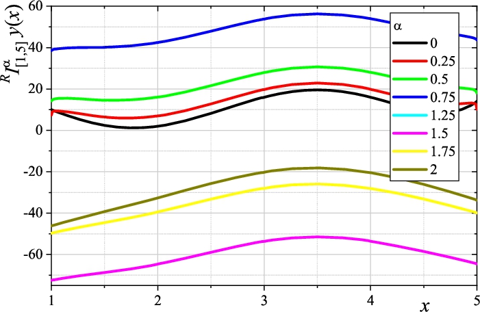
In Fig. 1, the plot of function (69) (which corresponds to $\alpha =0$) and the plots of the Riesz fractional integrals ${^{R}}{I_{[1,5]}^{\alpha }}y(x)$ (71) for $\alpha =0.25,0.5,0.75,1.25,1.5,1.75,2$ are shown. While, the numerical errors ${\textit{err}_{N}}$ obtained on the interval $[1,5]$ for $N=100,200,400,800,1600,3200,6400,12800$ and $\alpha =0.75$, for five considered methods are illustrated in the plots in Fig. 2. It can be seen for this considered problem that the error values can be both positive and negative, but errors always decrease as N increases.
Fig. 1
Plots of ${^{R}}{I_{[1,5]}^{\alpha }}y(x)$ for function (68) and $\alpha \in \{0,0.25,0.5,0.75,1.25,1.5,1.75,2\}$.
Example 4.
The last example concerns the comparison of the calculation results of the developed methods with an external approach. Here, we take into account the approximation method developed by Dimitrov (2021). His asymptotic expansion formula for the trapezoidal approximation of the left-sided fractional integral is as follows (the symbols in this formula have been adapted to the symbols used in this work)
where $\zeta (\cdot )$ is the Riemann zeta function.
(72)
\[\begin{aligned}{}{I_{{a^{+}}}^{\alpha }}y(x)& \simeq \frac{1}{\Gamma (\alpha )}\Bigg({(\Delta x)^{\alpha }}{\sum \limits_{k=1}^{N-1}}\frac{y(x-k\Delta x)}{{k^{1-\alpha }}}+\frac{y(a)}{2{(x-a)^{1-\alpha }}}\Delta x\\ {} & \hspace{1em}-\frac{(\alpha -1){(x-a)^{\alpha -2}}y(a)-{(x-a)^{\alpha -1}}{y^{\prime }}(a)}{12}{(\Delta x)^{2}}\\ {} & \hspace{1em}-\zeta (1-\alpha )y(x){(\Delta x)^{\alpha }}+\zeta (-\alpha ){y^{\prime }}(x){(\Delta x)^{\alpha +1}}\\ {} & \hspace{1em}-\zeta (-1-\alpha )\frac{{y^{\prime\prime }}(x)}{2}{(\Delta x)^{\alpha +2}}+\zeta (-2-\alpha )\frac{{y^{\prime\prime\prime }}(x)}{6}{(\Delta x)^{\alpha +3}}\Bigg)\\ {} & \hspace{1em}+\mathrm{O}\big({(\Delta x)^{4}}\big),\end{aligned}\]Based on one of the examples presented in Dimitrov (2021), we take function $y(x)=\exp (\lambda x)$, for which the analytical form of the left-sided fractional integral of order $\alpha \gt 0$ is the following
where ${E_{\alpha ,\beta }}(\cdot )$ is two-parameter Mittag-Leffler function (Kilbas et al., 2006) and λ is a constant.
(73)
\[ {I_{{a^{+}}}^{\alpha }}\exp (\lambda x)=\exp (\lambda a){(x-a)^{\alpha }}{E_{1,1+\alpha }}\big(\lambda (x-a)\big),\]Table 4 presents the errors ${\textit{err}_{N}}$ and the $\textit{EOC}$’s values calculated for three variants of the cubic splines, whereby the results for the Dimitrov’s method have been taken from his work (see: Dimitrov, 2021). The example calculations have been performed for $\lambda =1$, $\alpha =0.5$, $a=0$, $b=2$ and $N=40,80,160,320,640$. The analytical value of ${I_{{0^{+}}}^{0.5}}\exp (x){|_{x=2}}$ is also given in the table.
Table 4
Results related to Example 4.
| N | $\Delta x$ | Dimitrov’s method | Cubic spline | ||||||
| Variant 1 | Variant 2 | Variant 3 | |||||||
| ${\textit{err}_{N}}$ | $\textit{EOC}$ | ${\textit{err}_{N}}$ | $\textit{EOC}$ | ${\textit{err}_{N}}$ | $\textit{EOC}$ | ${\textit{err}_{N}}$ | $\textit{EOC}$ | ||
| 40 | 0.05 | no data | – | 4.87E−08 | – | 7.98E−08 | – | 1.66E−07 | – |
| 80 | 0.025 | 1.06E−09 | 4.04725 | 3.46E−09 | 3.81833 | 4.66E−09 | 4.09663 | 8.45E−09 | 4.29274 |
| 160 | 0.0125 | 6.48E−11 | 4.03414 | 2.27E−10 | 3.92785 | 2.76E−10 | 4.07693 | 4.44E−10 | 4.25181 |
| 320 | 0.00625 | 3.98E−12 | 4.02694 | 1.45E−11 | 3.96779 | 1.66E−11 | 4.05782 | 2.40E−11 | 4.20937 |
| 640 | 0.003125 | 2.34E−13 | 4.08360 | 9.17E−13 | 3.98378 | 1.01E−12 | 4.04244 | 1.33E−12 | 4.16883 |
| Analytical value of ${I_{{0^{+}}}^{0.5}}\exp (x){|_{x=2}}=7.052852096484309014376129$ (calculated using (73)) | |||||||||
As can be seen in Table 4, the results for all variants of the cubic splines and for the Dimitrov’s method have the identical $\textit{EOC}=4$, but for the same integration step sizes, the obtained numerical errors are slightly larger in the case of the cubic spline methods. As an explanation for the smaller error values in the Dimitrov’s article, one should delve into his method. Equation (72) contains the derivatives (up to the third order) of the integrand function. Knowledge of the analytical values of these derivatives at points a and x significantly improves the quality of numerical evaluation of the fractional integral in his developed method. His method can be considered a composition of the analytical and numerical approaches. Our computational schemes based on the cubic splines are purely numerical, and also the values of derivatives of the integrand function at the end point conditions are determined only numerically. Unfortunately, in the case of a very complicated form of the integrand function, it is often difficult to find the values of the first, second and third derivatives in an analytical way, and hence it can be problematic to use it for the Dimitrov’s method.
4 Conclusions
We have derived the numerical integration formulas for evaluating the fractional order integrals. These formulas are based on the interpolation of the integrand function by the linear, quadratic and cubic splines. The integration method that uses the linear spline (i.e. the piecewise linear function) is treated as a complement and is used to compare the obtained results with the methods that use the quadratic and cubic splines.
Analysing the results presented in all tables and graphs (as well as other performed results, but omitted and not presented in this work), it can be noticed that the calculated numerical values of the fractional order integrals have good agreement with the exact analytical solution (if this solution is known, of course), and the numerical errors ${\textit{err}_{N}}$ tend to 0 as the grid size N increases for all derived integration methods. We can see that as N increases, the values of the $\textit{EOC}$ are stabilized and tend to the specified values, and for different kinds of splines used we obtained: $\textit{EOC}=2$ for the linear spline, $\textit{EOC}=\min \{3+\alpha ,4\}$ for the quadratic spline, $\textit{EOC}=4$ for all variants of the clamped cubic splines. Here, one can observe the consistency of the obtained $\textit{EOC}$ values for the particular methods with the orders of error (defined by the O notation) which were estimated analytically. Moreover, analysing the numerical results (by comparing the order of numerical errors, as well as the $\textit{EOC}$) for three variants of the cubic splines, we can notice that these numerical methods have a similar order of errors, however, it can be seen that variant 1 generally generates slightly smaller errors. If we compare the order of numerical errors for methods using the quadratic and cubic splines (where the $EOC=4$ is the same), we can conclude that the quadratic spline gives worse results than the cubic splines.
From a computational point of view, in the case of the methods that use the clamped cubic splines (all variants), the linear system of equations needs to be solved, which can be computationally time consuming, and thus it has certain disadvantages of the methods as a result. But here, in the case of derived methods, we need only to solve a tri-diagonal system of equations, which can be solved easily and faster, e.g. by using the Thomas algorithm of complexity O(N). This problem does not occur in the case of the linear and quadratic splines where the coefficients of the interpolation spline are determined locally, and these algorithms can be easily parallelized.
Summing up, it can be said that the obtained numerical results for the derived integration methods that use the cubic or quadratic splines give higher values of the $\textit{EOC}$ than for the method that uses the linear splines. This confirms the efficiency and the applicability of the derived numerical algorithms for the fractional integration of function.


