1 Introduction
Virtual environments already became a part of our daily life including applied computer games, learning environments (Devlin
et al.,
2015), business and project management environment (Mattioli
et al.,
2015), social networks and their games. These applications and its multimedia elements are causing negative or positive emotions and are considered as a virtual stimuli (Wrzesien
et al.,
2015). These stimuli may be used as a clue to regulate human psychological, emotional and social state (Devlin
et al.,
2015) or even to treat various mental diseases (Calvo
et al.,
2015). For this purpose, a control mechanism for human state regulation or stabilization is needed.
EEG-based emotion signals (excitement, frustration, engagement/boredom) are characterized as reliable and quick response signals (Hondrou and Caridakis,
2012; Mattioli
et al.,
2015; Sourina and Liu,
2011). However, foremost we need to compose and investigate mathematical models describing dependencies between emotion signals as a reaction to stimuli.
Predictive input-output structure models were proposed and investigated for exploring dependencies between virtual 3D face features and human reaction to them when dynamic virtual 3D face is observed without a virtual reality headset (Kaminskas
et al.,
2014; Kaminskas and Vidugirienė,
2016; Vaškevičius
et al.,
2014). Predictive models are necessary in the design of predictor-based control systems (Astrom and Wittenmark,
1997; Clarke,
1994; Kaminskas,
2007). Predictor-based control was applied to the control of human emotion signals, when a dynamic 3D face is observed without a virtual reality headset (Kaminskas
et al.,
2015; Kaminskas and Ščiglinskas,
2016).
This paper introduces a predictor-based control with a generalized minimum variance control quality principles which are applied to the control of human response signal, when a dynamic virtual 3D face as stimuli is observed using a virtual reality headset.
2 Experiment Planning and Cross-Correlation Analysis
A virtual 3D face with changing distance-between-eyes was used for input and EEG-based pre-processed excitement signal of a volunteer was measured as output (Fig.
1). The output signal was recorded with Emotiv Epoc device. This device records EEG inputs from 14 channels (in accordance with the international 10–20 locations): AF3, F7, F3, FC5, T7, P7, O1, O2, P8, T8, FC6, F4, F8, AF4 (Emotiv Epoc specifications, Mattioli
et al. (
2015)). Values of the output signal (excitement) vary from 0 to 1. If excitement is low, the value is close to 0 and if it is high, the value is close to 1.

Fig. 1
Input–output scheme.
A dynamic stimulus was formed from a changing woman face (Kaminskas
et al.,
2015). A 3D face created with Autodesk MAYA was used as a “neutral” one (Fig.
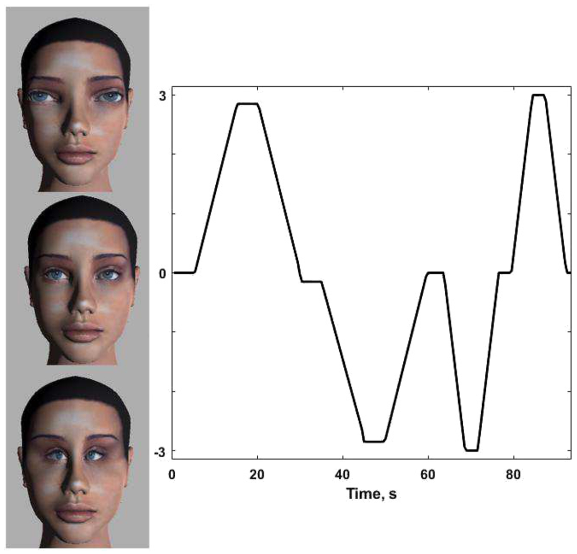
2, middle). Other 3D faces were formed by changing distance-between-eyes in an extreme manner (Fig.
2, top, bottom). The transitions between normal and extreme stages were programmed. “Neutral” face has 0 value, largest distance-between-eyes corresponds to value 3 and smallest distance-between-eyes corresponds to value – 3 (Fig.
2). At first “neutral” face was shown for 5 s, then the distance-between-eyes was increased continuously and in 10 s the largest distance between eyes was reached, then 5 s of steady face was shown and after that the face came back to “normal” state in 10 s. Then “normal” face was shown for 5 s, followed by 10 s of continuous change to the face with the smallest distance between-eyes, again 5 s of steady face was shown and in the next 10 s the face came back to “normal”. The experiment was continued in the same way further using 3 s time intervals for steady face and 5 s for continuous change. Eight volunteers (four males and four females) were tested. Each volunteer was watching a changing virtual 3D face with virtual reality headset and each experiment was approximately about 100 s long. EEG-based excitement and changing distance-between-eyes signals were measured with sampling period
${T_{0}}=0.5$ s and recorded in real time.

Fig. 2
Experiment plan for a stimulus – testing input.
To estimate the possible relation between human response (excitement) and virtual 3D face feature (distance-between-eyes) a cross-correlation analysis was performed. The estimates of the maximum cross-correlation function values
are shown in Table
1. In Eq. (
19)
${R_{yx}}[\tau ]$ is a cross-covariation function between distance-between-eyes (
x) and excitement (
y) signals, and
${R_{yy}}[\tau ]$,
${R_{xx}}[\tau ]$ are auto-covariation functions (Vaškevičius
et al.,
2014). Examples of cross-correlation functions are demonstrated in Fig.
3.
Table 1
Maximum cross-correlation function values.
| No. volunteer |
1 |
2 |
3 |
4 |
5 |
6 |
7 |
8 |
| Female |
Female |
Female |
Female |
Male |
Male |
Male |
Male |
| Max. values |
0.90 |
0.68 |
0.66 |
0.50 |
0.83 |
0.81 |
0.81 |
0.48 |
The shift of the maximum values of cross-correlation functions in relation to ${R_{yx}}[0]$ allows stating that there exists dynamic relationship between virtual 3D face feature (distance-between-eyes) and human response (excitement) to them. High cross-correlation values justify a possibility of linear dynamic relations.
4 Parameter Identification Method
The current estimates of the parameters can be obtained in the identification process from the condition (Kaminskas,
2007)
where
is a vector of the coefficients of the polynomials (
3) and
${\theta _{0}}$,
is one-step-ahead output prediction error,
is one-step-ahead output prediction model,
is stability domain (unity disk) for the model (
2),
${z_{i}^{A}}$ is the roots of the polynomial
z is a forward-shift operator (
$z{y_{t}}={y_{t+1}}$), T is a vector transpose sign, sign
$|.|$ denotes absolute value.
Predictive model (
8) can be expressed in the form of linear regression
where
Considering Eq. (
7) and Eq. (
11), identification criterion
is a quadratic form of the vector variable
c.
Accordingly, solution of the minimization problem (
5) is separated into two stages. In the first stage, which is application of the least squares method, parameter estimates are calculated without evaluation of restrictions
In the second stage, these estimates are projected into stability domain (
9)
where
is a diagonal block-matrix of projection of the dimension
$(m+n+2)\times (m+n+2)$,
${\mathbf{I}_{b}}$ and
${\mathbf{I}_{a}}$ are correspondingly unity matrix dimension
$(m+1)\times (m+1)$ and
$(n\times n)$.
Factor
γ in matrix (
16) is calculated by equation
where
${\gamma _{\mathrm{max}}}\| {\mathbf{c}_{t}}\| $ is the distance from the point
$\mathbf{0}$ (origin) to the boundary of stability domain
${\Omega _{\mathbf{c}}}$ in the direction of
${\mathbf{c}_{t}}$,
$\| .\| $ is the Euclidean norm sign,
${\gamma _{0}}$ is a small and positive constant. When
$n\leqslant 2$ (stability domain for the model (
2) is defined by linear inequations) factor
γ calculation was given (Kaminskas
et al.,
2014) and when
$n\leqslant 3$ (stability domain is defined by linear and quadratic inequations) factor
γ calculation was given (Kaminskas and Vidugirienė,
2016).
Estimates of the model orders
$(\hat{m},\hat{n})$ are defined from the following conditions (Kaminskas and Vidugirienė,
2016):
where
$\tilde{m}$ and
$\tilde{n}$ are polynomial (
3) degrees when the following inequalities are correct
$\sigma \epsilon [m,n]$ is one-step-ahead prediction error standard deviation for model order
$(m,n)$,
$\delta \epsilon [0.01,0.1]$ is chosen constant value (which corresponds to a relative variation of predictions error standard deviation from 1% to 10%).
Validation of the predictive models (
8) was performed for each of eight volunteers (four males and four females). For the identification of unknown parameters the first 60 to 100 observations were used for each volunteer. For evaluation of the model order and prediction accuracy all 185 observations were used. Each model is selected from twelve possible models (when
$n=1,2,3$,
$m=0,1,2,3$). The analysis of the experiment results showed relations between distance-between-eyes and excitement and it can be described using first order (
$\hat{m}=0$,
$\hat{n}=1$) model
Prediction accuracies with predictive model (
20) were correspondingly evaluated using the prediction error standard deviation, relative prediction error standard deviation and average absolute relative prediction error (Vaškevičius
et al.,
2014):
where
$N=185$. Parameter estimates and a predictor accuracy measures are provided in Table
2. Figures
4 and
5 show examples of one-step-ahead prediction results when we are using model (
20) for four volunteers.
Table 2
Estimatesof parameter and prediction accuracy measures.
| No. |
Volunteer |
${\hat{\theta }_{0}}$ |
${\hat{b}_{0}}$ |
${\hat{a}_{1}}$ |
${\sigma _{\varepsilon }}$ |
${\hat{\sigma }_{\varepsilon }}(\% )$ |
$\left|\bar{\varepsilon }\right|\left(\% \right)$ |
| 1 |
Female |
0.0383 |
−0.0115 |
−0.9431 |
0.0391 |
9.2 |
7.3 |
| 2 |
Female |
0.0042 |
0.0027 |
−0.9674 |
0.0150 |
10.0 |
7.2 |
| 3 |
Female |
0.0139 |
0.0060 |
−0.9244 |
0.0258 |
8.7 |
6.5 |
| 4 |
Female |
0.0383 |
−0.0142 |
−0.9152 |
0.0413 |
10.9 |
7.4 |
| 5 |
Male |
0.0056 |
−0.0061 |
−0.9935 |
0.0252 |
9.8 |
7.3 |
| 6 |
Male |
0.0152 |
−0.0104 |
−0.9833 |
0.0324 |
11.4 |
8.9 |
| 7 |
Male |
0.0014 |
−0.0028 |
−0.9972 |
0.0298 |
11.0 |
8.3 |
| 8 |
Male |
0.0162 |
−0.0064 |
−0.9698 |
0.0386 |
9.3 |
7.0 |
|
|
|
|
Average |
0.0309 |
10.0 |
7.5 |

Fig. 4
Example of one-step-ahead prediction results for female (right volunteer No. 1 and left No. 2).

Fig. 5
Example of one-step-ahead prediction results for male (right volunteer No. 5 and left No. 6).
The analysis of the identification results showed what relations between distance-between-eyes and excitement is described by first order (
$\hat{m}=0$,
$\hat{n}=1$) model (
20). The validation results show that excitement can be predicted on average with less than 8% average absolute relative prediction error. Accordingly, input-output structure model (
2), (
3) in the predictive form (
8) can be applied to the design of prediction-based control system of human excitement signal.
5 Generalized Minimum Variance Control
A predictor-based control law is synthesized by minimizing control quality criterion
${Q_{t}}$ (
${x_{t+1}}$) in an admissible domain
${\Omega _{x}}$ (Kaminskas,
2007)
where
E is an expectation operator,
${y_{t+1}^{\ast }}$ is a reference signal (reference trajectory for excitement signal),
${x_{\min }}$ and
${x_{\mathrm{max}}}$ are input signal boundaries (smallest and largest distance-between-eyes),
${\delta _{t}}>0$ are the restriction values for the change rate of the input signal, and sign
$|.|$ denotes absolute value,
$q\geqslant 0$ are weight coefficients.
Then solving the minimization problem (
24)–(
26) for one-step ahead prediction model (
8), the control law is described by equations:
If the roots of polynomial
are in the unity disk
then from (
28)–(
30) the following equation is correct
If a part or all of polynomial (
31) roots do not belong to the unity disk, weight factor
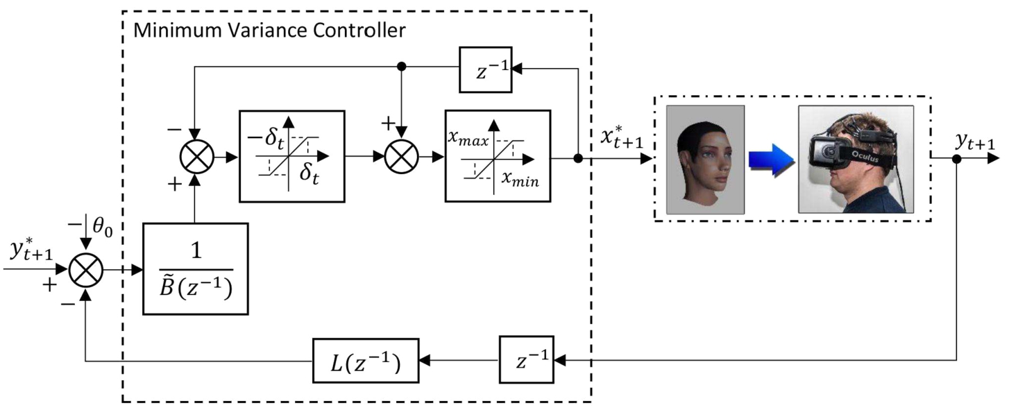
$|\lambda |$ is increased until all roots rely in the unity disk. The scheme of a generalized minimum variance controller (
27)–(
30) is illustrated in Fig.
6.

Fig. 6
The scheme of a generalized minimum variance control with constraints.
When inserting the control signal, which is described by equations (
28) and (
30), to the model (
2) we get a closed-loop system equation
It is clear from equation (
34), what stability of the closed-loop system is dependent of characteristic polynomial
roots, all the roots must be inside the unity disk
The analysis of characteristic polynomial equation (
35) allows to state what having stable model in the process of the identification (
5)–(
10), stability of a closed-loop system is obtained with any arrangement of roots of the polynomial
$B({z^{-1}})$, when the weight factor
$|\lambda |$ is increased.
From equation (
34) we get what permanent component of output signal in stationary regime (
${y_{t}^{\ast }}={y^{\ast }}$) is
where
is a gain of the transfer function of the reference signal
${y_{t}^{\ast }}$ in a closed – loop
Considering the expression (
38), weight factor
λ is calculated by equation
where
is a gain of the transfer function of the input-output model (
2)
From equation (
37) follows that sistematic control error
grows if
${K_{\mathrm{p}}}$ is significantly lower than unit (weight factor
$|\lambda |$ or weight coefficient
q in control criterion (
25) are high). Accordingly, the gain
${K_{\mathrm{p}}}$ is selected from an interval
or
When ${K_{\mathrm{p}}}=1$ ($\lambda =0$, $q=0$), we get a minimum variance control, in other cases we get a generalized minimum variance control.
Table 3
Efficiency measure of excitement control.
| No. |
Vol. |
${\delta _{t}}=12/s$ |
${\delta _{t}}=1.2/s$ |
${\delta _{t}}=0.3/s$ |
| ${K_{p}}$ |
1 |
0.9 |
0.8 |
1 |
0.9 |
0.8 |
1 |
0.9 |
0.8 |
| 1 |
Female |
51.1 |
48.9 |
45.2 |
36.8 |
33.9 |
16.0 |
32.0 |
34.8 |
33.1 |
| 2 |
Female |
86.3 |
83.4 |
77.6 |
83.7 |
82.5 |
77.6 |
80.2 |
77.6 |
77.6 |
| 3 |
Female |
33.6 |
32.6 |
30.6 |
31.2 |
31.1 |
29.3 |
27.8 |
24.0 |
27.4 |
| 4 |
Female |
39 |
35.8 |
31.9 |
27.9 |
17.5 |
31.4 |
27.9 |
16.2 |
14.1 |
| 5 |
Male |
192.8 |
159.1 |
121.8 |
128.6 |
158.7 |
121.7 |
132.0 |
158.9 |
121.1 |
| 6 |
Male |
161.2 |
149.0 |
103.3 |
131.0 |
122.7 |
103.3 |
37.6 |
72.5 |
103.2 |
| 7 |
Male |
122.8 |
118.4 |
113.1 |
107.1 |
118.2 |
112.6 |
96.0 |
98.2 |
96.9 |
| 8 |
Male |
65.2 |
61.3 |
57.6 |
48.9 |
27.5 |
50.3 |
27.3 |
43.3 |
55.9 |
|
Average |
94 |
86.1 |
72.6 |
74.4 |
74.0 |
67.8 |
57.6 |
65.7 |
66.2 |
Modelling experiments consisted of two phases. In the first phase a human excitement signal as a response to dynamical 3D face stimuli (testing input) were observed. According with these observations parameter estimates of the predictive model (
20) were calculated using identification. In the second phase, dynamical virtual 3D face features were formed according with the control law (
27) and (
33) (control output). The control tasks were to maintain high excitement levels (reference signals). In this case a control efficiency can be evaluated by a relative measure
where
${\bar{y}_{T}}$ is an average of output
${y_{t}^{T}}$ (excitement) as a response to testing input, and
${\bar{y}_{c}}$ is an average of output
${y_{t}^{c}}$ (excitement) as a response to control input. These measures are given in Table
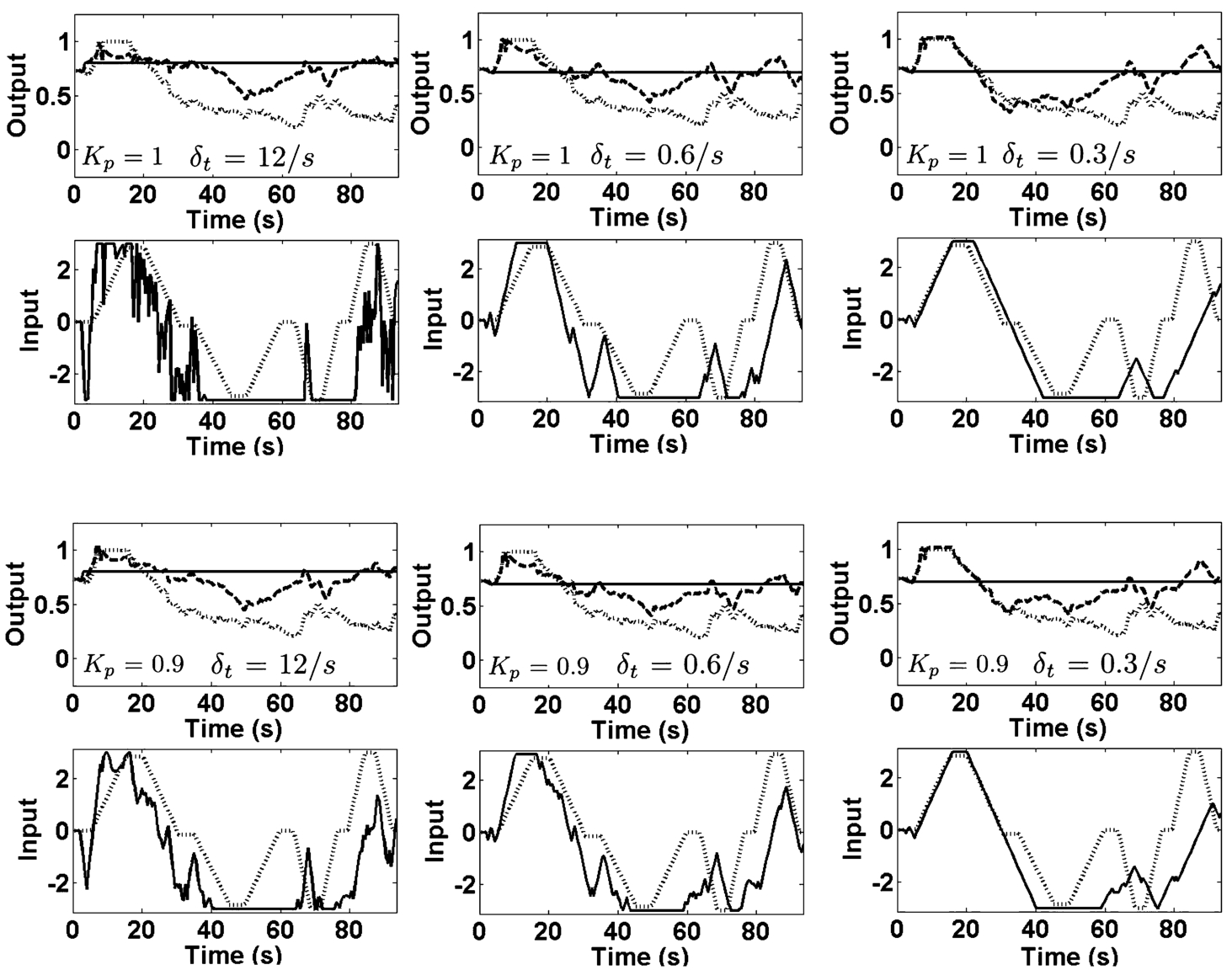
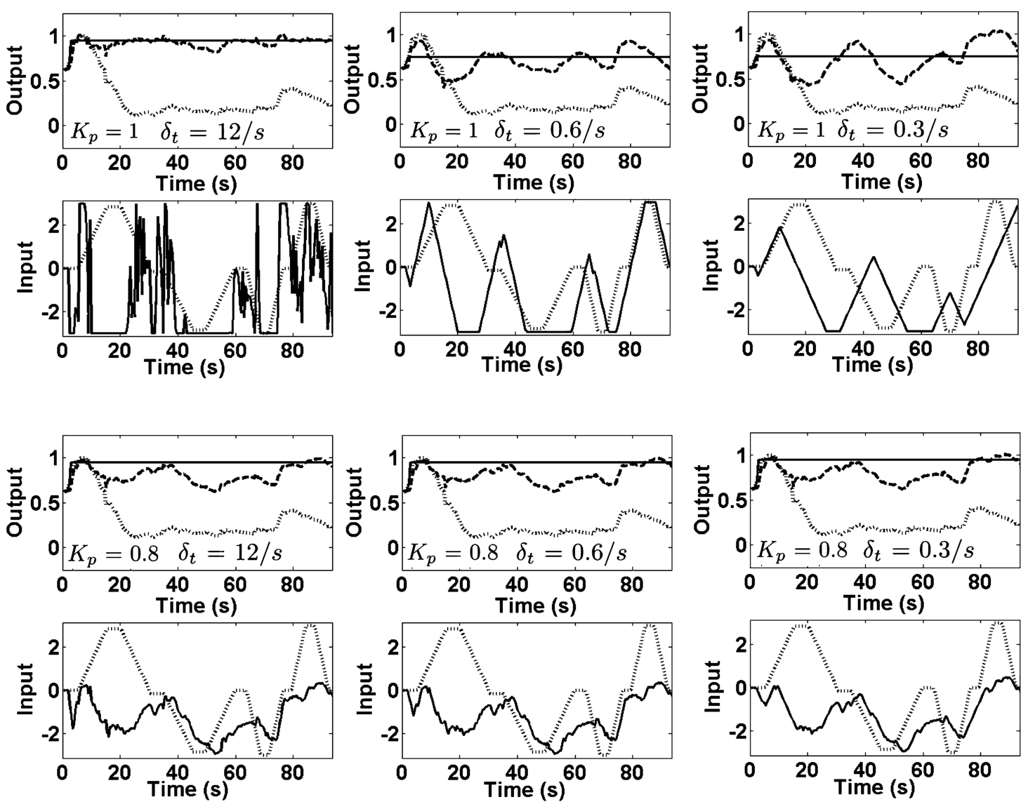
3. Examples of excitement control results are shown in Fig.
7 and Fig.
8 (weight factor
$\lambda =-0.0224$ and weight coefficient
$q=0.00026$, when
${K_{p}}=0.9$ or
$\lambda =-0.2346$,
$q=0.00143$, when
${K_{p}}=0.8$).

Fig. 7
Examples of excitement control for volunteer No. 1 (female). Output: reference signal ${y_{t}^{\ast }}$ (solid line), output signals ${y_{t}^{c}}$ (dotted line) and ${y_{t}^{T}}$ (dashed line). Input: control signal ${x_{t}^{\ast }}$ (solid line) and testing input ${x_{t}}$ (dashed line).
Modelling results show that using predictor-based control with constraints a sufficiently good quality of human excitement signal control can be reached. Excitement signal level can be raised up on average to about 95% (when ${K_{\mathrm{p}}}=1$, minimum variance control) and about 85%–70% (when ${K_{\mathrm{p}}}=0.9$ and ${K_{\mathrm{p}}}=0.8$, generalized minimum variance control) in comparison with testing input.

Fig. 8
Examples of excitement control for volunteer No. 5 (male). Output: reference signal ${y_{t}^{\ast }}$ (solid line), output signals ${y_{t}^{c}}$ (dotted line) and ${y_{t}^{T}}$ (dashed line). Input: control signal ${x_{t}^{\ast }}$ (solid line) and testing input ${x_{t}}$ (dashed line).
Control quality is influenced by a control signal variation speed which is limited by the parameter
${\delta _{t}}$ of the admissible domain. This parameter allows decreasing control signal variation which is usually high in minimum variance control systems without constraints. Control signal variation decreases when a generalized minimum variance control is applied. In this case, the quality of control depends on a gain coefficient in closed-loop
${K_{\mathrm{p}}}$ (
38), whose value defines weight factor
λ in (
30) or weight coefficient
q in control criterion (
25).
6 Conclusions
Experiment planning and cross-correlation analysis results demonstrated that there is a relatively high correlation between 3D face features observed using virtual reality (distance-between-eyes) and human response (excitement) to the stimuli. The shift of the maximum values of the cross-correlations functions in relation to origin allows stating that there exists linear dynamic relationship between distance-between-eyes and excitement signals. Parameter identification method for building stable input-output structure model is proposed. Identification and validation results of one-step-ahead prediction model (
8) show that excitement can be predicted on average with less than 8% average absolute relative prediction error.
Accordingly, input-output structure model (
2) (
3) in the predictive form (
8) can be applied to the design of predictor-based control system for controlling human excitement signal as a response to a dynamic virtual 3D face. Control law is synthesized by minimizing generalized minimum variance control criterion in an admissible domain for input. Calculation method of weight factor
λ in control law (
27)–(
30) or weight coefficient
q in control criterion (
25) is proposed. This method is based on admissable value of the systematic control error.
Sufficiently good control quality of excitement signal, maintained signal level is at average to about 90% (when
${K_{\mathrm{p}}}=1$, minimum variance control) and about 70% (when
${K_{\mathrm{p}}}=0.8$, generalized minimum variance control with high weight coefficient) higher compared to testing input, is demonstrated by modelling results. Experiment results demonstrated possibility to decrease variations of the control signal using a limited signal variation speed when decreasing constant
${\delta _{t}}$ in expression (
27) or using a generalized minimum variance control when increasing weight factor
$|\lambda |$, which is calculated according to equation (
40). However, in these cases, particularly applying minimum variance control, control quality decreases.

