Informatica logo


Login Register

  1. Home
  2. Issues
  3. Volume 31, Issue 4 (2020)
  4. Robust Dynamic Programming in N Players ...

Informatica

Information Submit your article For Referees Help ATTENTION!
  • Article info
  • Full article
  • Related articles
  • More
    Article info Full article Related articles

Robust Dynamic Programming in N Players Uncertain Differential Games
Volume 31, Issue 4 (2020), pp. 769–791
Manuel Jiménez-Lizárraga   Sara V. Rodríguez-Sánchez   Naín de la Cruz   César Emilio Villarreal  

Authors

 
Placeholder
https://doi.org/10.15388/20-INFOR436
Pub. online: 23 November 2020      Type: Research Article      Open accessOpen Access

Received
1 July 2019
Accepted
1 November 2020
Published
23 November 2020

Abstract

In this paper we consider a non-cooperative N players differential game affected by deterministic uncertainties. Sufficient conditions for the existence of a robust feedback Nash equilibrium are presented in a set of min-max forms of Hamilton–Jacobi–Bellman equations. Such conditions are then used to find the robust Nash controls for a linear affine quadratic game affected by a square integrable uncertainty, which is seen as a malicious fictitious player trying to maximize the cost function of each player. The approach allows us to find robust strategies in the solution of a group of coupled Riccati differential equation. The finite, as well as infinite, time horizon cases are solved for this last game. As an illustration of the approach, the problem of the coordination of a two-echelon supply chain with seasonal uncertain fluctuations in demand is developed.

1 Introduction

Differential games stand as a suitable framework for modelling strategic interaction between different agents (known as players), where each of them is looking for the minimization or, equivalently, the maximization of his individual criterion (Engwerda, 2005; Başar and Olsder, 1999). In such a multi-player scenario, none of the players is allowed to maximize his profits or objectives at the expense of the rest of the players. Therefore, the solution of the game is given in a form of “equilibrium of forces”.
Among different types of solutions, the so called Nash equilibrium is the most extensively used in the game theory literature. In this solution none of the players can improve their criteria by unilaterally deviating from their Nash strategy; therefore, no player has an incentive to change his decision. When the full state information is available to all the players to realize their decision strategy in each point of time, this is called a feedback Nash equilibrium (Engwerda, 2005; Başar and Olsder, 1999; Friedman, 1971). In order to find such feedback strategies, the optimal control tools are applied, specifically an equivalent N players form of the Hamilton–Jacobi–Bellman equation is required to be solved for each of the players. In the case of the non-cooperative Nash equilibrium solution framework, each player deals with a single criterion optimization problem (the standard optimal control problem), with the actions of the remaining players taking fixed equilibrium values.
Although the notion of robustness is such an important feature in the control theory, there are not many studies of dynamic games that are affected by some sort of uncertainties or disturbances. Some recent developments on this topic can be mentioned. Jiménez-Lizárraga and Poznyak (2007) presented a notion of open loop Nash equilibrium (OLNE) where the parameters of the game are within a finite set and the solution is given in terms of the worst-case scenario, that is, the result of the application of certain control input (in terms of the cost function value) is associated with the worst or least favourable value of the unknown parameter. The article of Jank and Kun (2002) shows also an OLNE and derives conditions for the existence and uniqueness of a worst case Nash equilibrium (WCNE); however, in this case they considered that the uncertainty belongs to a Hilbert functional space and enters adding up into the time derivative of the state variables. A similar problem is considered in a quite recent work (Engwerda, 2017), where the author shows that the WCNE can be derived by finding an ONLE of an associated differential game with $2N$ initial state constraints, the author derives necessary and sufficient conditions for the solution of the finite time problem. The work of Jungers et al. (2008) deals with a game with polytopic uncertainties that reformulated the problem as a nonconvex coupling between semi-definite programming to find the Nash type controls. Other related approaches include: using the Nash strategy to design robust controls for linear systems (Chen and Zhou, 2001). Another way to deal with uncertainties is to view them as an exogenous input (a fictitious player) (Chen et al., 1997). In the work of van den Broek et al. (2003) the definition of equilibria is extended to deal with two cases: a soft-constrained formulation whose basis is given by Jank and Kun (2002), where the fictitious player is introduced in the criteria via a weighting matrix.
In this work, inspired in the works of Jank and Kun (2002) and Engwerda (2005, 2017), we analyse a deterministic N-player non-zero sum Differential Game case, considering finite, as well as infinite, time horizon in the performance index and a ${L^{2}}$ perturbation which is considered as a fictitious player trying to maximize the cost of each i-th player.
Assuming the player has access to the full state information, we are interested in finding a type of robust feedback Nash strategies, that guarantee a robust equilibrium when the players consider the worst case of the perturbation with respect to their own point of view. To that end, a set of robust form of the HJB equations are introduced; each of these equations compute not only the minimum of the i-th player control; but the maximum or worst case uncertainty from his point of view; resulting in a min-max form of the known HJB equations for a N players game. To the best of the authors’ knowledge, using such a robust HJB equation has not been considered before to find a robust feedback Nash equilibrium in linear quadratic deterministic games, which stand as an important case to study. To summarize, the contributions of this work are as follows:
  • 1. Presentation of the general conditions of robust worst case feedback Nash equilibrium by means of a robust form of the HJB equation for N players non-zero sum games.
  • 2. Based on such a formulation, it gives the solution for the finite time horizon for the linear affine quadratic uncertain game.
  • 3. It gives the solution of the infinite horizon for the linear affine dynamics.
  • 4. It illustrates the result solving a problem of coordination of a two-echelon supply chain with seasonal uncertain fluctuations in demand. Such a case has not been treated before.
The development of this paper is as follows. In Section 2 we state, formally, the general problem of a differential game and the conditions for the Robust Nash Equilibrium to exist. Then, in Section 3 we define the dynamics of the problem analysed and the type of functional cost we have to minimize for a finite time horizon problem, we also state a theorem based on dynamic programming to find the robust controls for each player. In Section 4 we analyse the case of infinite time horizon. Finally, Section 5 follows with a numerical example. The purpose of this last section is to show how to apply the formulas obtained in Sections 3–4 and then compare our results against a finite time differential game which does not consider perturbation in the solution of the problem, which is the common problem treated, but the system itself is affected by some sort of perturbation.

2 Problem Statement

In this section we exploit the principle of dynamic programming in order to find all the robust feedback Nash equilibrium strategies for each player of a Non-zero sum uncertain differential game. We begin by presenting the general sufficient conditions for such a robust equilibrium to exist. Towards that end, consider the following N-person uncertain differential game with initial pair $(s,y)\in [0,T]\times {\mathbb{R}^{n\times 1}}$ described by the following initial value problem
(1)
\[ \begin{aligned}{}& \dot{x}(t)=f\big(x(t),\big({u_{1}}(t),{u_{2}}(t),\dots ,{u_{N}}(t)\big),w(t),t\big),\hspace{1em}x(s)=y,\\ {} & \text{a.e.}\hspace{2.5pt}\hspace{2.5pt}t\in [s,T],\hspace{1em}T<+\infty ,\end{aligned}\]
where $x(t)\in {\mathbb{R}^{n\times 1}}$ is the state column vector of the game and ${u_{i}}(t)\in {\mathbb{R}^{{l_{i}}\times 1}}$ is the control strategy at time t for each player i that may run over a given control region ${U_{i}}\subset {\mathbb{R}^{{l_{i}}\times 1}}$, i represents the number of player for $i\in \{1,\dots ,N\}$, ${u_{\hat{\imath }}}$ is the vector of strategies for the rest of the players, $\hat{\imath }$ is the counter-coalition of players counteracting the player with index i and $w(t)\in {\mathbb{R}^{q\times 1}}$ is a finite unknown disturbance in the sense that ${\textstyle\int _{0}^{T}}\| w(t){\| ^{2}}\mathrm{d}t<+\infty $, that is, w is square integrable or, stated another way, $w\in {L^{2}}[0,T]$. The cost function as individual aim performance
(2)
\[ {J_{i}}(s,y,{u_{i}},{u_{\hat{\imath }}},w):={\int _{s}^{T}}{g_{i}}\big(x(t),{u_{i}}(t),{u_{\hat{\imath }}}(t),w(t),t\big)\mathrm{d}t+{h_{i}}\big(x(T)\big),\]
which contains the integral term as well as a terminal state is given in the standard Bolza form.
Throughout the article we shall use the next notations:
  • • ${^{A}}B$ is the set of functions from the set A to the set B.
  • • ${A^{\mathrm{t}}}$ is the transpose of the matrix A.
  • • ${I_{N,i}}:=\{k\in \mathbb{N}:1\leqslant k\leqslant N$ and $k\ne i\}$.
  • • ${\mathcal{U}_{\mathrm{adm}}^{i}}[{s_{0}},{s_{1}}]:=\{{u_{i}}{\in ^{[{s_{0}},{s_{1}}]}}{U_{i}}:{u_{i}}$ is measurable}.
  • • ${\mathcal{U}_{\mathrm{adm}}^{i}}:={\mathcal{U}_{\mathrm{adm}}^{i}}[0,T]$ is the set of all admissible control strategies.
  • • ${\mathcal{U}_{\mathrm{adm}}^{\hat{\imath }}}:={\mathcal{U}_{\mathrm{adm}}^{1}}\times \cdots \times {\mathcal{U}_{\mathrm{adm}}^{i-1}}\times {\mathcal{U}_{\mathrm{adm}}^{i+1}}\times \cdots \times {\mathcal{U}_{\mathrm{adm}}^{N}}$.
  • • ${\mathcal{U}_{\mathrm{adm}}}:{=✕_{i=1}^{N}}{\mathcal{U}_{\mathrm{adm}}^{i}}$.
  • • If $u\in {\mathcal{U}_{\mathrm{adm}}}$, for $t\in [0,T]$, $u(t):=({u_{1}}(t),{u_{2}}(t),\dots ,{u_{N}}(t))$.
  • • ${\mathrm{D}_{i}}f$ denotes the partial derivative of f with respect to the i-th component.
  • • ${\mathbb{1}_{A}}$ denotes the indicator function of a set A.
Hypothesis 1.
The control region ${U_{i}}$ is a subset of ${\mathbb{R}^{{l_{i}}\times 1}}$. The maps f, ${g_{i}}$ and ${h_{i}}$ are such that for all $({u_{i}},{u_{\hat{\imath }}},w)\in {\mathcal{U}_{\mathrm{adm}}^{i}}\times {\mathcal{U}_{\mathrm{adm}}^{\hat{\imath }}}\times {L^{2}}[0,T]$, equation (1) admits an a.e. unique solution and the function ${J_{i}}$ given in (2) is well defined; in general we assume the conditions given by Yong and Zhou (1999, p. 159).
Remark 1.
We assume that the integrand ${g_{i}}$ given in Equation (2) is positive definite, then the cost function ${J_{i}}$ could not take negative values.

2.1 Robust Feedback Nash Equilibrium

Next, we introduce the worst case uncertainty from the point of view of the i-th player according to the complete set of controls ${u_{j}}$, with $j\in \{1,\dots ,N\}$ (Jank and Kun, 2002; Engwerda, 2017):
(3)
\[ {J_{i}}\big(s,y,{u_{i}},{u_{\hat{\imath }}},{w_{i,{u_{i}},{u_{\hat{\imath }}}}^{\ast }}\big):=\underset{w\in {L^{2}}[s,T]}{\max }{J_{i}}(s,y,{u_{i}},{u_{\hat{\imath }}},w).\]
In this paper we want to extend the robust Nash equilibrium notion, previously introduced by Jank and Kun (2002) for an open loop information structure, to a full state feedback information for an N players game.
Definition 1.
The control strategies ${u_{1}^{\mathrm{rn}}},{u_{2}^{\mathrm{rn}}},\dots ,{u_{N}^{\mathrm{rn}}}$, are said to be robust feedback Nash equilibrium, where ${({u_{i}^{\mathrm{rn}}},)_{i=1}^{N}}\in {\mathcal{U}_{\mathrm{adm}}}$, if for any vector of admissible strategies
\[ ({u_{i}},{u_{\hat{\imath }}})\in {\mathcal{U}_{\mathrm{adm}}^{i}}\times {\mathcal{U}_{\mathrm{adm}}^{\hat{\imath }}},\hspace{1em}\text{for}\hspace{2.5pt}i\in \{1,\dots ,N\},\]
assuming the existence of the corresponding maximizing uncertainty function ${w_{i,{u_{i}},{u_{\hat{\imath }}^{\mathrm{rn}}}}^{\ast }}\in {L^{2}}[0,T]$ from the point of view of the i-th player. Then, we have the next set of inequalities:
(4)
\[ {J_{i}}\big(s,y,{u_{i}^{\mathrm{rn}}},{u_{\hat{\imath }}^{\mathrm{rn}}},{w_{i,{u_{i}^{\mathrm{rn}}},{u_{\hat{\imath }}^{\mathrm{rn}}}}^{\ast }}\big)\leqslant {J_{i}}\big(s,y,{u_{i}},{u_{\hat{\imath }}^{\mathrm{rn}}},{w_{i,{u_{i}},{u_{\hat{\imath }}^{\mathrm{rn}}}}^{\ast }}\big).\]
In those conditions, we say also that $({u_{1}^{\mathrm{rn}}},{u_{2}^{\mathrm{rn}}},\dots ,{u_{N}^{\mathrm{rn}}})$ is a vector of robust feedback Nash strategies for the whole set of players.
Hypothesis 2.
There is a unique vector of robust feedback Nash strategies for the whole set of players.
Now in order to find the robust feedback Nash equilibrium control strategies for the problem given by (2) subject to (1), we consider the following definition.
Definition 2.
Consider the N-tuples of strategies $({u_{1}},{u_{2}},\dots ,{u_{N}})$ and the robust value function for the i-th player as:
(5)
\[ \begin{aligned}{}& {V_{i}}(s,y):=\underset{{u_{i}}\in {U_{i}}}{\min }\hspace{0.1667em}{J_{i}}\big(s,y,{u_{i}},{u_{\hat{\imath }}^{\mathrm{rn}}},{w_{i,{u_{i}},{u_{\hat{\imath }}^{\mathrm{rn}}}}^{\ast }}\big),\hspace{1em}\text{for}\hspace{2.5pt}i\in \{1,2,\dots ,N\},\\ {} & {V_{i}}\big(T,x(T)\big):={h_{i}}\big(x(T)\big),\end{aligned}\]
for any particular initial pair $(s,y)\in [0,T)\times {\mathbb{R}^{n\times 1}}$. The function ${V_{i}}$ is also called the robust Bellman function.
Remark 2.
Notice that the minimization operation over ${u_{i}}$ considers that the rest of the players are fixed in their Robust strategies (4) and each ${w_{i,{u_{i}},{u_{\hat{\imath }}}}^{\ast }}$ satisfies (3).

2.2 Robust Dynamic Programming Equation

Let us explore the Bellman principle of optimality (Poznyak, 2008) for the robust value function ${V_{i}}$ associated with the min-max posed problem for the i-th player, considering the rest of the participants as well as the signal function w fixed.
For ${u_{i}}\in {\mathcal{U}_{\mathrm{adm}}^{i}}$, let us take ${v_{i}}={\mathbb{1}_{[s,\hat{s})}}{u_{i}}+{\mathbb{1}_{[\hat{s},T)}}{u_{i}^{\mathrm{rn}}}$ and note that ${v_{i}}\in {\mathcal{U}_{\mathrm{adm}}^{i}}$. Using the Bellman principle of optimality for the functional ${J_{i}}(s,y,{v_{i}},{u_{\hat{\imath }}^{\mathrm{rn}}},\cdot )$, where ${J_{i}}$ is given in equation (2), and using also equation (5) given in Definition 2 we have:
(6)
\[\begin{aligned}{}{V_{i}}(s,y)& \leqslant {J_{i}}\big(s,y,{v_{i}},{u_{\hat{\imath }}^{\mathrm{rn}}},{w_{i,{v_{i}},{u_{\hat{\imath }}^{\mathrm{rn}}}}^{\ast }}\big)=\underset{w\in {L^{2}}[s,T]}{\max }{J_{i}}\big(s,y,{v_{i}},{u_{\hat{\imath }}^{\mathrm{rn}}},w\big)\\ {} & =\underset{w\in {L^{2}}[s,T]}{\max }\Bigg\{{\int _{s}^{\hat{s}}}{g_{i}}\big(x(t),{u_{i}}(t),{u_{\hat{\imath }}^{\mathrm{rn}}}(t),w(t),t\big)\mathrm{d}t\\ {} & \hspace{1em}+{\int _{\hat{s}}^{T}}{g_{i}}\big(x(t),{u_{i}^{\mathrm{rn}}}(t),{u_{\hat{\imath }}^{\mathrm{rn}}}(t),w(t),t\big)\mathrm{d}t+{h_{i}}\big(x(T)\big)\Bigg\}\\ {} & =\underset{w\in {L^{2}}[s,T]}{\max }\Bigg\{{\int _{s}^{\hat{s}}}{g_{i}}\big(x(t),{u_{i}}(t),{u_{\hat{\imath }}^{\mathrm{rn}}}(t),w(t),t\big)\mathrm{d}t+{V_{i}}\big(\hat{s},x(\hat{s})\big)\Bigg\},\end{aligned}\]
where the control strategies ${u_{\hat{\imath }}^{\mathrm{rn}}}$ are robust Nash controls defined in (4) and $x(\hat{s})$ is such that x fulfills (1) when ${u_{j}}={u_{j}^{\mathrm{rn}}}$ for $j\ne i$ and $w={w_{i,{u_{i}},{u_{\hat{i}}^{\mathrm{rn}}}}^{\ast }}$ that is described in the Definition 1. Hence, taking the minimum in the right part of (6) over ${u_{i}}$, the inequality yields to
(7)
\[\begin{aligned}{}rl{V_{i}}(s,y)& \leqslant \underset{{u_{i}}\in {\mathcal{U}_{\mathrm{adm}}^{i}}[s,T]}{\min }\underset{w\in {L^{2}}[s,T]}{\max }\Bigg\{{\int _{s}^{\hat{s}}}{g_{i}}\big(x(t),{u_{i}}(t),{u_{\hat{\imath }}^{\mathrm{rn}}}(t),w(t),t\big)\mathrm{d}t\\ {} & \hspace{1em}+{V_{i}}\big(\hat{s},x(\hat{s})\big)\Bigg\}.\end{aligned}\]
On the other hand, beside for any $\delta >0$, there is a control ${u_{i,\delta }}\in {\mathcal{U}_{\mathrm{adm}}^{i}}$, with the property:
(8)
\[ {V_{i}}(s,y)+\delta \geqslant \underset{w\in {L^{2}}[s,T]}{\max }\Bigg\{{\int _{s}^{\hat{s}}}{g_{i}}\big({x_{\delta }}(t),{u_{i,\delta }}(t),{u_{\hat{\imath }}^{\mathrm{rn}}}(t),w(t),t\big)\mathrm{d}t+{V_{i}}\big(\hat{s},{x_{\delta }}(\hat{s})\big)\Bigg\},\]
where ${x_{\delta }}$ is the solution of (1) under the application of the control ${u_{i,\delta }}$ keeping the rest of the players fixed. Indeed, if there is a $\delta >0$ such that for any ${u_{i}}\in {\mathcal{U}_{\mathrm{adm}}^{i}}$ we have
\[ {V_{i}}(s,y)+\delta <\underset{w\in {L^{2}}[s,T]}{\max }\Bigg\{{\int _{s}^{\hat{s}}}{g_{i}}\big(x(t),{u_{i}}(t),{u_{\hat{\imath }}^{\mathrm{rn}}}(t),w(t),t\big)\mathrm{d}t+{V_{i}}\big(\hat{s},x(\hat{s})\big)\Bigg\},\]
then, taking ${u_{i}}={u_{i}^{\mathrm{rn}}}$ and using the Bellman principle of optimality, we would obtain
\[\begin{aligned}{}{V_{i}}(s,y)+\delta & <\underset{w\in {L^{2}}[s,T]}{\max }\Bigg\{{\int _{s}^{\hat{s}}}{g_{i}}\big(x(t),{u_{i}^{\mathrm{rn}}}(t),{u_{\hat{\imath }}^{\mathrm{rn}}}(t),w(t),t\big)\mathrm{d}t+{V_{i}}\big(\hat{s},x(\hat{s})\big)\Bigg\}\\ {} & \leqslant \underset{w\in {L^{2}}[s,T]}{\max }\Bigg\{{\int _{s}^{\hat{s}}}{g_{i}}\big(x(t),{u_{i}^{\mathrm{rn}}}(t),{u_{\hat{\imath }}^{\mathrm{rn}}}(t),w(t),t\big)\mathrm{d}t\\ {} & \hspace{1em}+{\int _{\hat{s}}^{T}}{g_{i}}\big(x(t),{u_{i}^{\mathrm{rn}}}(t),{u_{\hat{\imath }}^{\mathrm{rn}}}(t),{w_{i,{u_{i}^{\mathrm{rn}}},{u_{\hat{\imath }}^{\mathrm{rn}}}}^{\ast }}(t),t\big)\mathrm{d}t+{h_{i}}\big(x(T)\big)\Bigg\}\\ {} & ={V_{i}}(s,y),\end{aligned}\]
arriving to a contradiction. So, from the inequality (8) we get
(9)
\[\begin{aligned}{}{V_{i}}(s,y)+\delta & \geqslant \underset{w\in {L^{2}}[s,T]}{\max }\Bigg\{{\int _{s}^{\hat{s}}}{g_{i}}\big({x_{\delta }}(t),{u_{i,\delta }}(t),{u_{\hat{\imath }}^{\mathrm{rn}}}(t),w(t),t\big)\mathrm{d}t+{V_{i}}\big(\hat{s},{x_{\delta }}(\hat{s})\big)\Bigg\}\\ {} & \geqslant \underset{{u_{i}}\in {\mathcal{U}_{\mathrm{adm}}^{i}}[s,T]}{\min }\underset{w\in {L^{2}}[s,T]}{\max }\Bigg\{{\int _{s}^{\hat{s}}}{g_{i}}\big(x(t),{u_{i}}(t),{u_{\hat{\imath }}^{\mathrm{rn}}}(t),w(t),t\big)\mathrm{d}t\\ {} & \hspace{1em}+{V_{i}}\big(\hat{s},x(\hat{s})\big)\Bigg\}.\end{aligned}\]
Now, as in the inequality (9), the value of δ is positive, but arbitrary, we have
(10)
\[\begin{aligned}{}{V_{i}}(s,y)& \geqslant \underset{{u_{i}}\in {\mathcal{U}_{\mathrm{adm}}^{i}}[s,T]}{\min }\underset{w\in {L^{2}}[s,T]}{\max }\Bigg\{{\int _{s}^{\hat{s}}}{g_{i}}\big(x(t),{u_{i}}(t),{u_{\hat{\imath }}^{\mathrm{rn}}}(t),w(t),t\big)\mathrm{d}t\\ {} & \hspace{1em}+{V_{i}}\big(\hat{s},x(\hat{s})\big)\Bigg\}\end{aligned}\]
(Fattorini, 1999; Poznyak, 2008).
From the inequalities (7) and (10), we have arrived to the next theorem that is a robust form of the dynamic programming equation, for the problem in consideration.
Theorem 1.
Let the basic assumption of Section 2 hold, then for any initial pair $(s,y)\in [0,T)\times {\mathbb{R}^{n\times 1}}$, the following relationship holds:
(11)
\[\begin{aligned}{}{V_{i}}(s,y)& =\underset{{u_{i}}\in {\mathcal{U}_{\mathrm{adm}}^{i}}[s,T]}{\min }\underset{w\in {L^{2}}[s,T]}{\max }\Bigg\{{\int _{s}^{\hat{s}}}{g_{i}}\big(x(t),{u_{i}}(t),{u_{\hat{\imath }}^{\mathrm{rn}}}(t),w(t),t\big)\mathrm{d}t\\ {} & \hspace{1em}+{V_{i}}\big(\hat{s},x(\hat{s})\big)\Bigg\},\end{aligned}\]
for all $\hat{s}\in [s,T]$.
The development of the principle of optimality to equation (11), leads immediately to the following result:
Theorem 2.
Let’s consider the uncertain affine N-players differential game given by (1)–(2), where T is finite and the full state information is known. In this case the vector of control strategies $({u_{i}^{\mathrm{rn}}},{u_{\hat{\imath }}^{\mathrm{rn}}})$ provides a robust feedback equilibrium if there exists a continuously differentiable function ${V_{i}}:[0,T]\times {\mathbb{R}^{n\times 1}}\to \mathbb{R}$ satisfying the following partial differential equation:
(12)
\[\begin{aligned}{}& -{\mathrm{D}_{1}}{V_{i}}\big(t,x(t)\big)=\underset{{u_{i}}\in {\mathcal{U}_{\mathrm{adm}}^{i}}}{\min }\underset{w\in {L^{2}}[s,T]}{\max }\big\{{\mathrm{D}_{2}}{V_{i}}{\big(t,x(t)\big)^{\mathrm{t}}}\hspace{2.5pt}f\big(x(t),{\hat{u}_{i}}(t),w(t),t\big)\\ {} & \phantom{-{\mathrm{D}_{1}}{V_{i}}\big(t,x(t)\big)=}+{g_{i}}\big(x(t),{u_{i}}(t),{u_{\hat{\imath }}^{\mathrm{rn}}}(t),w(t),t\big)\big\};\\ {} & {V_{i}}\big(T,x(T)\big)={h_{i}}\big(x(T)\big),\hspace{1em}\textit{for}\hspace{2.5pt}i\in \{1,\dots ,N\},\end{aligned}\]
where $\hat{{u_{i}}}(t)=({u_{1}^{\mathrm{rn}}}(t),\dots ,{u_{i-1}^{\mathrm{rn}}}(t),{u_{i}}(t),{u_{i+1}^{\mathrm{rn}}}(t),\dots ,{u_{N}^{\mathrm{rn}}}(t))$, and the corresponding min-max cost for each player is
(13)
\[ {J_{i}^{\ast }}={V_{i}}(s,y).\]
Remark 3.
The partial differential equation (12) of Theorem 2 is called the robust Hamilton–Jacobi–Bellman (RHJB) equation. In previous important works dealing with the design of robust ${H_{\infty }}$ controllers using a dynamic game approach (Başar and Bernhard, 2008; Aliyu, 2011) the min-max version of the value function was already found. It was also found that actually when all the players are fixed in their robust Nash controls the game became a zero-sum game, played out between the i-th player and the uncertainty. Equation (12) is an extension to the N players non-zero sum game; however, to the best of our knowledge, this case has not been introduced yet.

3 Finite Time Horizon N Players Linear Affine Quadratic Differential Game

Once the general conditions for the existence of a robust feedback Nash equilibrium in an uncertain differential game are established, we turn now to the special case of the linear affine quadratic differential games (LAQDG). In this section we consider the case where the time horizon is finite, that is, $T<+\infty $. The game is played by N participants which are trying to minimize certain loss inflicted by a disturbance, besides, the functional cost of the game is restricted by the corresponding differential equation. Therefore, in this section we assume that:
(14)
\[ \begin{aligned}{}& f\big(x(t),u(t),w(t),t\big):=A(t)x(t)+{\sum \limits_{j=1}^{N}}{B_{j}}(t){u_{j}}(t)+E(t)\hspace{0.1667em}w(t)+c(t),\\ {} & x(t)\in {\mathbb{R}^{n\times 1}},\hspace{2em}x(0)={x_{0}},\hspace{2em}{u_{j}}(t)\in {\mathbb{R}^{{l_{j}}\times 1}},\hspace{1em}0\leqslant t\leqslant T<+\infty \end{aligned}\]
the functions for the cost of each player are given by the following quadratic functions:
(15)
\[ \begin{aligned}{}{g_{i}}\big(x(t),{u_{i}}(t),{u_{\hat{\imath }}}(t),w(t),t\big)& :=x{(t)^{\mathrm{t}}}{Q_{i}}(t)x(t)\\ {} & \hspace{1em}+{\sum \limits_{j=1}^{N}}{u_{j}}{(t)^{\mathrm{t}}}{R_{i,j}}(t){u_{j}}(t)-w{(t)^{\mathrm{t}}}{W_{i}}(t)w(t),\\ {} {h_{i}}\big(x(T)\big)& :=x{(T)^{\mathrm{t}}}{Q_{i\mathrm{f}}}x(T),\end{aligned}\]
where j represents the number of the player, $A(t)\in {\mathbb{R}^{n\times n}}$, and ${B_{j}}(t)\in {\mathbb{R}^{n\times {l_{j}}}}$, for $j\in \{1,\dots ,N\}$, are the known system and controls matrices; $x(t)$ is the state vector of the game and ${u_{j}}$ is the control strategy for the j-th player; $c(t)\in {\mathbb{R}^{n\times 1}}$ is an exogenous and known signal. In this case w is the same as in (1), that is, a finite disturbance entering the system through the matrix $E(t)\in {\mathbb{R}^{n\times q}}$. The performance index for each i-th player is given again in standard Bolza form, the strategy for the player i is ${u_{i}}$ while ${u_{\hat{\imath }}}$ are the strategies of the rest of the players. The term $w{(t)^{\mathrm{t}}}{W_{i}}(t)w(t)$ is the unknown uncertainty, which is trying to maximize the cost ${J_{i}}$ from the point of view of the i-th player. The cost matrices are assumed to satisfy: ${Q_{i}}(t)={Q_{i}}{(t)^{\mathrm{t}}}\geqslant \mathbf{0}$, ${Q_{i\mathrm{f}}}={Q_{i\mathrm{f}}^{\mathrm{t}}}\geqslant \mathbf{0}$ and ${W_{i}}(t)={W_{i}}{(t)^{\mathrm{t}}}>\mathbf{0}$ (symmetric and semipositive/positive definite matrices); ${R_{i,i}}(t)={R_{i,i}}{(t)^{\mathrm{t}}}>\mathbf{0}$ and ${R_{i,j}}(t)={R_{i,j}}{(t)^{\mathrm{t}}}\geqslant \mathbf{0}$, where inequalities mean inequalities component by component. Assume also that the players have access to the full state information pattern, that is, they measure $x(t)$, for all $t\in [0,T]$. All the involved squared matrices are assumed to be non-singular.
For the linear affine dynamics given in (14), equation (12) can be rewritten as follows:
(16)
\[\begin{aligned}{}-{\mathrm{D}_{1}}{V_{i}}\big(t,x(t)\big)& =\underset{{u_{i}}\in {\mathcal{U}_{\mathrm{adm}}^{i}}}{\min }\hspace{2.5pt}\hspace{2.5pt}\hspace{2.5pt}\underset{w\in {L^{2}}[0,T]}{\max }\bigg\{{\mathrm{D}_{2}}{V_{i}}{\big(t,x(t)\big)^{\mathrm{t}}}\bigg(A(t)x(t)+{B_{i}}(t){u_{i}}(t)\\ {} & \hspace{1em}+\sum \limits_{j\in {I_{N,i}}}{B_{j}}(t){u_{j}^{\mathrm{rn}}}(t)+E(t)w(t)+c(t)\bigg)\\ {} & \hspace{1em}+x{(t)^{\mathrm{t}}}{Q_{i}}(t)x(t)+{u_{i}}{(t)^{\mathrm{t}}}{R_{i,i}}(t){u_{i}}(t)\\ {} & \hspace{1em}+\sum \limits_{j\in {I_{N,i}}}{u_{j}^{\mathrm{rn}}}{(t)^{\mathrm{t}}}{R_{i,j}}(t){u_{j}^{\mathrm{rn}}}(t)-w{(t)^{\mathrm{t}}}{W_{i}}(t)w(t)\bigg\}\end{aligned}\]
with terminal condition as ${V_{i}}(T,x(T))=x{(T)^{\mathrm{t}}}{Q_{i\mathrm{f}}}x(T)$. With this condition and if the assumptions mentioned above are satisfied, the Robust Feedback Nash Equilibrium can be directly obtained as
(17)
\[\begin{aligned}{}{u_{i}^{\mathrm{rn}}}& =\arg \underset{{u_{i}}\in {\mathcal{U}_{\mathrm{adm}}^{i}}}{\min }\bigg\{{\mathrm{D}_{2}}{V_{i}}{\big(\cdot ,x(\cdot )\big)^{\mathrm{t}}}\bigg(Ax+{B_{i}}{u_{i}}+\sum \limits_{j\in {I_{N,i}}}{B_{j}}{u_{j}}+E{w_{i,{u_{i}},{u_{\hat{\imath }}^{\mathrm{rn}}}}^{\ast }}+c\bigg)\\ {} & \hspace{1em}+{x^{\mathrm{t}}}{Q_{i}}x+{u_{i}^{\mathrm{t}}}{R_{i,i}}{u_{i}}+\sum \limits_{j\in {I_{N,i}}}{{u_{j}^{\mathrm{rn}}}^{\mathrm{t}}}{R_{i,j}}{u_{j}^{\mathrm{rn}}}-{{w_{i,{u_{i}},{u_{\hat{\imath }}^{\mathrm{rn}}}}^{\ast }}^{\mathrm{t}}}{W_{i}}\hspace{0.1667em}{w_{i,{u_{i}},{u_{\hat{\imath }}^{\mathrm{rn}}}}^{\ast }}\bigg\},\end{aligned}\]
and worst case uncertainty from the point of view of the i-th player is obtained as
(18)
\[\begin{aligned}{}{w_{i,{u_{i}},{u_{\hat{\imath }}}}^{\ast }}& =\arg \underset{w\in {L^{2}}[0,T]}{\max }\Bigg\{{\mathrm{D}_{2}}{V_{i}}{\big(\cdot ,x(\cdot )\big)^{\mathrm{t}}}\Bigg(Ax+{\sum \limits_{j=1}^{N}}{B_{j}}{u_{j}}+Ew+c\Bigg)\\ {} & \hspace{1em}+{x^{\mathrm{t}}}{Q_{i}}x+{\sum \limits_{j=1}^{N}}{u_{j}^{\mathrm{t}}}{R_{i,j}}{u_{j}}-{w^{\mathrm{t}}}{W_{i}}w\Bigg\}.\end{aligned}\]
Remark 4.
Notice that the value of ${w_{i,{u_{i}},{u_{\hat{\imath }}}}^{\ast }}$ given in (18) does not depend of $({u_{i}},{u_{\hat{\imath }}})$. So, in this particular case, we shall denote such value just by ${w_{i}^{\ast }}$.
Theorem 3.
The robust feedback Nash strategies for the uncertain LQ affine game (14)–(15), has the next linear form:
(19)
\[ {u_{i}^{\mathrm{rn}}}=-{R_{i,i}^{-1}}{B_{i}^{\mathrm{t}}}({P_{i}}x+{m_{i}})\]
and the worst case uncertainty from the point of view of the i-th player is:
(20)
\[ {w_{i}^{\ast }}={W_{i}^{-1}}{E_{i}^{\mathrm{t}}}({P_{i}}x+{m_{i}}),\]
where the set of N Riccati type coupled equations ${P_{i}}$ satisfy the following boundary value problem:
(21)
\[\begin{aligned}{}& -{\dot{P}_{i}}={\tilde{A}^{\mathrm{t}}}{P_{i}}+{P_{i}}\tilde{A}+Q-{P_{i}}{S_{i}^{\mathrm{t}}}{P_{i}}+{P_{i}}{M_{i}}{P_{i}}+\sum \limits_{j\in {I_{N,i}}}{P_{j}}{S_{j,i}}{P_{j}};\\ {} & {P_{i}}(T)={Q_{i\mathrm{f}}},\\ {} & \tilde{A}:=A-{\sum \limits_{j=1}^{N}}{S_{j}}{P_{j}},\end{aligned}\]
where ${S_{i}}:={B_{i}}{R_{i,i}^{-1}}{B_{i}^{\mathrm{t}}}$, ${S_{j,i}}:={B_{j}}{R_{j,j}^{-1}}{R_{i,j}}{R_{j,j}^{-1}}{B_{j}^{\mathrm{t}}}$, ${M_{i}}:=E{W_{i}^{-1}}{E^{\mathrm{t}}}$, for $i,j\in \{1,\dots ,N\}$; and the ${m_{i}}$ are the “shifting vectors” governed by the following coupled linear differential equations:
(22)
\[\begin{aligned}{}-{\dot{m}_{i}}& ={A^{\mathrm{t}}}\hspace{0.1667em}{m_{i}}-{P_{i}}\hspace{0.1667em}{S_{i}}\hspace{0.1667em}{m_{i}}-\sum \limits_{j\in {I_{N,i}}}{P_{i}}{S_{j}}\hspace{0.1667em}{m_{j}}-\sum \limits_{j\in {I_{N,i}}}{P_{j}}{S_{j}}\hspace{0.1667em}{m_{i}}\\ {} & \hspace{1em}+{P_{i}}{M_{i}}{m_{i}}+{P_{i}}c+\sum \limits_{j\in {I_{N,i}}}{P_{j}}{S_{j,i}}\hspace{0.1667em}{m_{j}};\hspace{1em}{m_{i}}(T)=0,\end{aligned}\]
and the value of the robust Nash cost is:
(23)
\[\begin{aligned}{}{J_{i}^{\ast }}& =x{(0)^{\mathrm{t}}}{P_{i}}x(0)+2{m_{i}}{(0)^{\mathrm{t}}}x(0)+{\int _{0}^{T}}\bigg({m_{i}^{\mathrm{t}}}{S_{i}}\hspace{0.1667em}{m_{i}}-2\sum \limits_{j\in {I_{N,i}}}{m_{i}^{\mathrm{t}}}{S_{j}}\hspace{0.1667em}{m_{j}}+{m_{i}^{\mathrm{t}}}{M_{i}}{m_{i}}\\ {} & \hspace{1em}+\sum \limits_{j\in {I_{N,i}}}{m_{j}^{\mathrm{t}}}{P_{j}}{S_{j,i}}\hspace{0.1667em}{P_{j}}{m_{j}}+2{m_{i}^{\mathrm{t}}}c\bigg),\end{aligned}\]
where ${J_{i}^{\ast }}$ is the optimum value of (2).
The proof of this theorem is presented in Appendix A.

4 Infinite Time Horizon Case

In this section we consider the same linear affine quadratic game when the time horizon is infinite. As the case analysed in the last section, the players are trying to minimize certain loss inflicted by a disturbance, besides, the functional cost of the game is restricted by a differential equation which considers an affine term. In this type of game the functional cost is given by:
(24)
\[ {J_{i}}(t,x,{u_{i}},{u_{\hat{\imath }}},w)={\int _{0}^{+\infty }}\Bigg({x^{\mathrm{t}}}{Q_{i}}x+{\sum \limits_{j=1}^{N}}{u_{j}^{\mathrm{t}}}{R_{j,i}}{u_{j}}-{w^{\mathrm{t}}}{W_{i}}w\Bigg),\]
and the constraint has the following form:
(25)
\[ \dot{x}(t)=Ax(t)+{\sum \limits_{j=1}^{N}}{B_{j}}{u_{j}}(t)+Ew(t)+c(t).\]
The involved matrices are constant with corresponding dimension and involved matrices in (24), satisfy equivalent restriction of the finite time counterpart. Following Engwerda (2005), we assume that $c\in {L_{\mathrm{exp},\hspace{0.1667em}\mathrm{loc}}^{2}}$, that is, locally square integrable and converging to zero exponentially. In this case, the system of algebraic Riccati equations takes on the form:
(26)
\[ {\tilde{A}^{\mathrm{t}}}{P_{i}}+{P_{i}}\tilde{A}+Q-{P_{i}}\hspace{0.1667em}{S_{i}^{\mathrm{t}}}\hspace{0.1667em}{P_{i}}+{P_{i}}{M_{i}}{P_{i}}+\sum \limits_{j\in {I_{N,i}}}{P_{j}}\hspace{0.1667em}{S_{j,i}}\hspace{0.1667em}{P_{j}}=0,\]
where $\tilde{A}:=A-{\textstyle\sum _{j=1}^{N}}{S_{j}}\hspace{0.1667em}{P_{j}}$.
To find the solution to this problem the completion of the square method is developed in Poznyak (2008) and the following theorem is stated.
Theorem 4.
For the differential game problem given by the equations (24)–(25), if the algebraic Riccati equations (26) possess symmetric stabilizing solutions ${P_{i}}$, then the infinite time horizon Robust Nash Equilibrium strategies are given by
(27)
\[ {u_{i}}(t)=-{R_{i,i}^{-1}}{B_{i}^{\mathrm{t}}}\big({P_{i}}x(t)+{m_{i}}(t)\big),\]
and the worst case will be given by
(28)
\[ {w_{i}}(t)={T_{i}^{-1}}{E^{\mathrm{t}}}\big({P_{i}}x(t)+{m_{i}}(t)\big),\]
where each ${m_{i}}$ fulfills the equation
(29)
\[ {m_{i}}(t)={\int _{t}^{+\infty }}\big({\mathrm{e}^{-({A_{i}}-{\textstyle\textstyle\sum _{j\ne i}^{N}}({P_{j}}{S_{j,i}}-{P_{i}}{S_{j}}))(t-s)}}{P_{i}}c(s)\big)\mathrm{d}s,\]
and
\[ {A_{i}}={A^{\mathrm{t}}}-{\sum \limits_{j=1}^{N}}{P_{j}}{S_{j}}+{\sum \limits_{j=1}^{N}}{P_{j}}{S_{j,i}}+{P_{i}}{M_{i}}.\]
Moreover, the optimal value ${J_{i}^{\ast }}$ is given by
(30)
\[ {J_{i}^{\ast }}=x{(0)^{\mathrm{t}}}{P_{i}}x(0)+2{m_{i}}{(0)^{\mathrm{t}}}x(0)+{n_{i}}(0)\]
and the closed loop states equation has the form
(31)
\[ \dot{x}(t)=\Bigg(A-{\sum \limits_{j=1}^{N}}{B_{j}}{R_{j,j}^{-1}}{B_{j}^{\mathrm{t}}}{P_{j}}\Bigg)x(t)-{\sum \limits_{j=1}^{N}}{B_{j}}{R_{j,j}^{-1}}{B_{j}^{\mathrm{t}}}{m_{j}}(t)+Ew(t)+c(t).\]
The proof of this theorem is found in Appendix A.

5 Numerical Example: A Differential Game Model for a Vertical Marketing System with Demand Fluctuation and Seasonal Prices

Consider a noncooperative game in a two-echelon supply chain established between two chain agents (Dockner et al., 2000; Jørgensen, 1986); a single supplier (called the manufacturer) and a single distributor (called the retailer). The manufacturer is in charge of selling a product type to a single retailer over a period of time T at the price ${p_{1}}(t)$. The retailer is in charge of distributing and marketing that product, at a price ${p_{2}}(t)={p_{1}}(t)+{r_{2}}(t)$, where ${r_{2}}(t)$ represents the profit margin gained by the retailer at time t per each unit sold. In this case, let us set ${r_{2}}=0.2{p_{1}}$.
The dynamic of the game is established by both players searching for a Nash equilibrium in their coordination contract, and furthermore facing some source of uncertainties. For this particular case assume that the retailer deals with a demand that evolves exogenously over time, with the quantity sold per time unit, d, depending not only on price ${p_{1}}$, but also on the time t elapsed, $d=d(p,t)$. The exogenous change in demand presented here is due to seasonal fluctuations. Under such enviroment, the profit equations for each players are ${J_{1}}$ and ${J_{2}}$ with the following quadratic structure:
(32)
\[\begin{aligned}{}& {J_{1}}={F_{1f}}{x_{1}^{2}}(26)+{\int _{0}^{26}}\bigg(\frac{{c_{1}}(t)}{2}{u_{1}^{2}}(t)+\frac{{h_{1}}}{2}{x_{1}^{2}}(t)\bigg)\mathrm{d}t,\end{aligned}\]
(33)
\[\begin{aligned}{}& {J_{2}}={F_{2f}}{x_{2}^{2}}(26)+{\int _{0}^{26}}\bigg(-{p_{2}}{w^{2}}(t)+\bigg(\frac{{p_{1}}+{c_{2}}(t)}{2}\bigg){u_{2}^{2}}(t)+\frac{{h_{2}}}{2}{x_{2}^{2}}(t)\bigg)\mathrm{d}t,\end{aligned}\]
subject to the following dynamic
(34)
\[\begin{aligned}{}& {\dot{x}_{1}}={u_{1}}-{u_{2}},\\ {} & {\dot{x}_{2}}={u_{2}}-d-ew,\end{aligned}\]
where ${J_{1}}$ indicates the operating cost faced by the manufacturer given by the holding cost and the production cost, plus a small penalization of the inventories at the final time of the horizon. On the other hand, ${J_{2}}$ indicates the operating cost incurred in by the retailer obtained by the holding cost, the production cost (including the price paid to the manufacturer for the products), and the perturbation signal w seen as a malicious fictitious player, and a small penalization of the inventories at the final time of the horizon. This game involves the dynamic changes of the inventory for each player $({x_{1}},{x_{2}})$, with the production rate $({u_{1}},{u_{2}})$ as decision variables. Moreover, the retailer’s dynamic faces an uncertain demand represented by two terms, the deterministic demand d plus the uncertain factor ew.
\[\begin{aligned}{}& A=\left(\begin{array}{c@{\hskip4.0pt}c}0\hspace{1em}& 0\\ {} 0\hspace{1em}& 0\end{array}\right),\hspace{1em}{B_{1}}=\left(\begin{array}{c}1\\ {} 0\end{array}\right),\hspace{1em}{B_{2}}=\left(\begin{array}{c}-1\\ {} 1\end{array}\right),\hspace{1em}D=\left(\begin{array}{c}0\\ {} -d\end{array}\right),\\ {} & {F_{1f}}=\left(\begin{array}{c@{\hskip4.0pt}c}8\hspace{1em}& 0\\ {} 0\hspace{1em}& 0\end{array}\right),\hspace{1em}{F_{2f}}=\left(\begin{array}{c@{\hskip4.0pt}c}0\hspace{1em}& 0\\ {} 0\hspace{1em}& 8\end{array}\right),\hspace{1em}E=\left(\begin{array}{c}0\\ {} 1\end{array}\right),\hspace{1em}{R_{11}}=\frac{{c_{1}}}{2},\\ {} & {R_{22}}=\frac{{p_{1}}+{c_{2}}}{2},\hspace{1em}{Q_{1}}=\left(\begin{array}{c@{\hskip4.0pt}c}\frac{{h_{1}}}{2}\hspace{1em}& 0\\ {} 0\hspace{1em}& 0\end{array}\right),\hspace{1em}{Q_{2}}=\left(\begin{array}{c@{\hskip4.0pt}c}0\hspace{1em}& 0\\ {} 0\hspace{1em}& \frac{{h_{2}}}{2}\end{array}\right),\end{aligned}\]
where
\[ {c_{1}}=0.85{p_{1}},\hspace{1em}{p_{2}}=2{p_{1}},\hspace{1em}{c_{2}}=2,\hspace{1em}{h_{1}}=15,\hspace{1em}{h_{2}}=10.5,\]
(35)
\[\begin{aligned}{}& {p_{1}}(t)=\left\{\begin{array}{l@{\hskip4.0pt}l}\frac{1}{5}(6t+90)\hspace{1em}& \text{for}\hspace{2.5pt}0\leqslant t\leqslant 5,\\ {} -3t+39\hspace{1em}& \text{for}\hspace{2.5pt}5<t\leqslant 6,\\ {} \frac{9}{2}t-6\hspace{1em}& \text{for}\hspace{2.5pt}6<t\leqslant 8,\\ {} -15t+150\hspace{1em}& \text{for}\hspace{2.5pt}8<t\leqslant 9,\\ {} \frac{20}{3}t-45\hspace{1em}& \text{for}\hspace{2.5pt}9<t\leqslant 12,\end{array}\right.\end{aligned}\]
(36)
\[\begin{aligned}{}& d(t)=\left\{\begin{array}{l@{\hskip4.0pt}l}-5{p_{1}}(t)+135\hspace{1em}& \text{for}\hspace{2.5pt}0\leqslant t<5,\\ {} -12{p_{1}}(t)+303\hspace{1em}& \text{for}\hspace{2.5pt}5<t\leqslant 6,\\ {} -\frac{26}{9}{p_{1}}(t)+\frac{1005}{9}\hspace{1em}& \text{for}\hspace{2.5pt}6<t\leqslant 8,\\ {} -\frac{37}{15}{p_{1}}(t)+\frac{1485}{15}\hspace{1em}& \text{for}\hspace{2.5pt}8<t\leqslant 9,\\ {} -5{p_{1}}(t)+135\hspace{1em}& \text{for}\hspace{2.5pt}9<t\leqslant 12.\end{array}\right.\end{aligned}\]
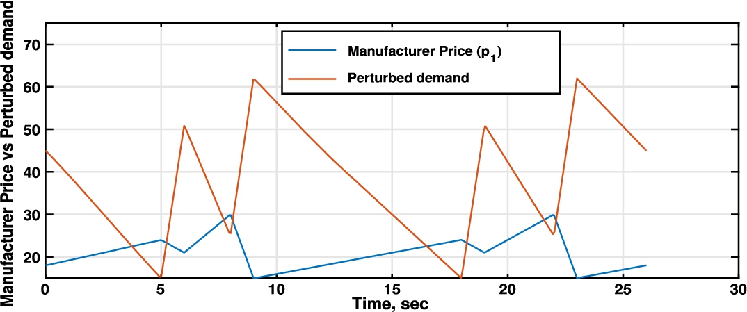
infor436_g001.jpg
Fig. 1
Price vs Perturbed demand.
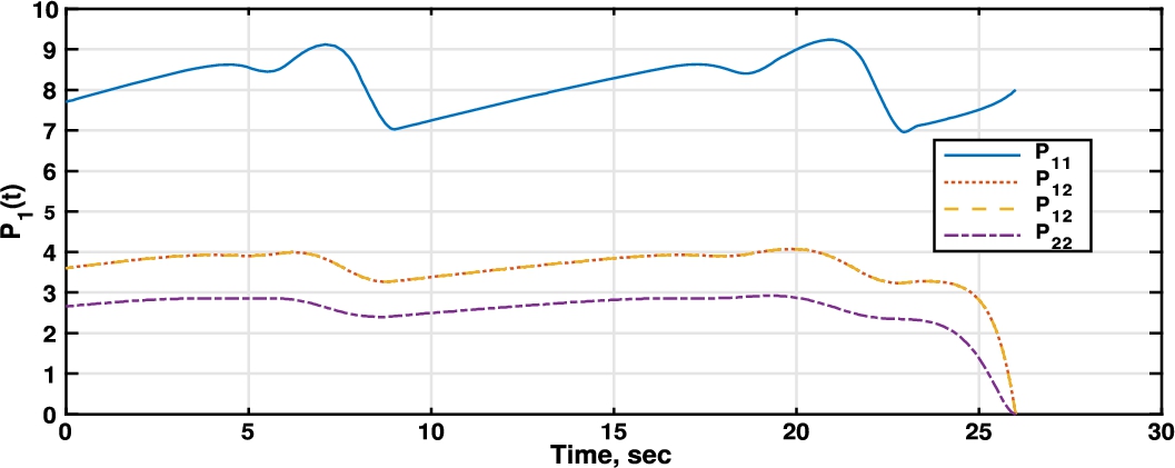
infor436_g002.jpg
Fig. 2
Riccati differential equation player 1 (manufacturer).
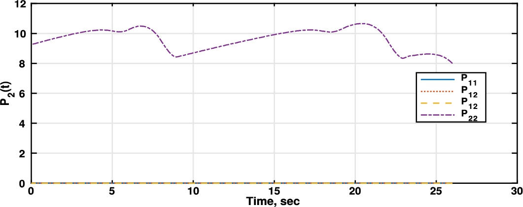
infor436_g003.jpg
Fig. 3
Riccati differential equation player 2 (retailer).
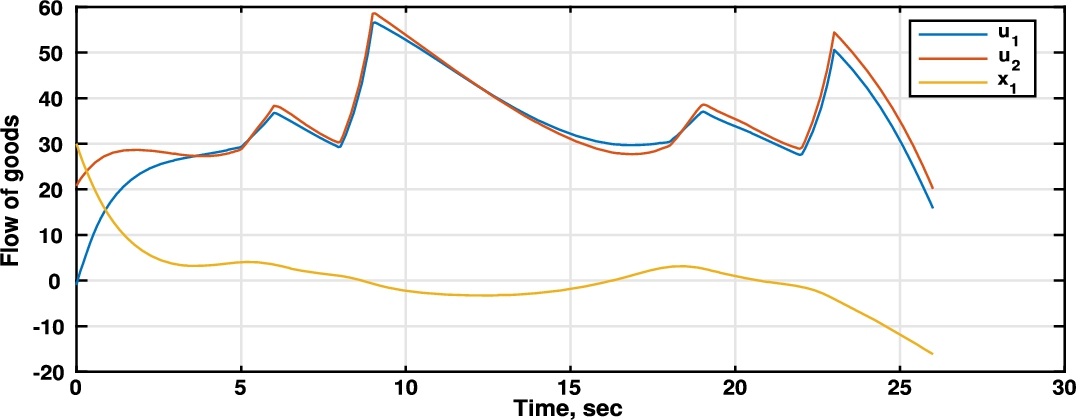
infor436_g004.jpg
Fig. 4
Comparison between manufacturer produced units (${u_{1}}$), units demanded by the retailer (${u_{2}}$), and units left in the manufacturer stock ${x_{1}}$.
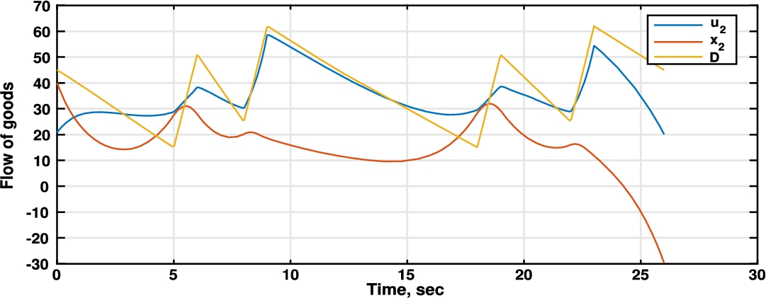
According to the game equations (1) and (2), $N=2$. We used the Matlab software to solve numerically backward in time (21), thus obtaining the corresponding robust Nash equilibrium strategies for each player. The results of such numerical solution are shown in figures (Figs. 2, 3). In Fig. 1 are depicted the perturbed demand and the manufacturer price. Figure 4 shows the behaviour of decision variables from each player, and the state equation from the manufacturer (${u_{1}}$ production manufacturer’s rate, ${u_{2}}$ purchasing retailer’s rate, and manufacturer’s inventory). Through this figure we can compare the different outputs, for instance, we observe that products left in the manufacturer’s stock basically are close to zero. In fact, this figure shows the advantages of better coordination between the different chain agents, in order to reduce bullwip effect. Since, the manufacturer and the retailer share information about customer demand, the produced goods from the manufacturer and the purchased goods from the retailer are deriving in similar behaviour.
Also, since there are no restrictions for the states of a given stage in the chain we can see that, at times, we are going to have negative values for this variable. For example, between $t=8$ and $t=16$, the units left in stock get a negative value, this only means that the manufacturer has backlogged units. However, we can appreciate that the amount of this backlogged units is minimum. Also for the closing of the season, between $t=20$ and $t=25$ it is better for the manufacturer only to have backlogged units. Once we get a Nash equilibrium, any deviation from the output policies would result in a loss for the manufacturer or the retailer.
infor436_g005.jpg
Fig. 5
Comparison between retailer bought units (${u_{2}}$), units demanded by the final consumer (D), and units left in the retailer stock (${x_{2}}$).
On the other hand, Fig. 5 shows the behaviour of the retailer’s dynamics through the time horizon. We can appreciate that the strategy followed by the retailer differs from the manufacturer in that the retailer uses inventory to face demand uncertainties. The retailer is considering the worst case of any perturbation on demand, but stock units are kept up to the minimum. The decisions at the end of the planning horizon are perturbed by the finite time horizon condition. For that reason the planning horizon was extended to two years in order to avoid such perturbations in the first year.

6 Conclusions

We found the Nash equilibrium control function of an N players differential game affected by an ${L^{2}}$ uncertainty function for a linear quadratic affine performance function in two cases:
  • 1. When we have a finite time horizon. In this case we assume the matrices involved in the performance function are time dependent.
  • 2. When we have an infinite time horizon. In this case we assume the matrices involved in the performance function are constant with respect to the time, and there are only temporal dependence of the uncertainty function, the state function, and an affine term of the constraint given by the linear differential equation.
Both problems are solved in this work using different methods.

A Appendix

Proof.
Proof of Theorem 3. To start the proof we find ${u_{i}^{\mathrm{rn}}}$ by means of (17) and the fact that
(37)
\[ \begin{aligned}{}{\mathrm{D}_{2}}{V_{i}}\big(t,x(t)\big)\big({B_{i}}(t)\big)+2{u_{i}}{(t)^{\mathrm{t}}}{R_{i,i}}(t)& =0\\ {} \Rightarrow {u_{i}}(t)=-\frac{1}{2}{R_{i,i}^{-1}}(t){B_{i}}{(t)^{\mathrm{t}}}{\big({\mathrm{D}_{2}}{V_{i}}\big(t,x(t)\big)\big)^{\mathrm{t}}},\end{aligned}\]
and we find ${w_{i}^{\ast }}$, given in Remark 4 by means of (18) and the fact that
(38)
\[ \begin{aligned}{}{\mathrm{D}_{2}}{V_{i}}\big(t,x(t)\big)\big(E(t)\big)+2w{(t)^{\mathrm{t}}}W(t)& =0\\ {} \Rightarrow w(t)=\frac{1}{2}{W_{i}^{-1}}(t)E{(t)^{\mathrm{t}}}{\big({\mathrm{D}_{2}}{V_{i}}(t,x)\big)^{\mathrm{t}}}.\end{aligned}\]
Substituting (37) and (38) back in (16) we get
(39)
\[\begin{aligned}{}-{\mathrm{D}_{1}}{V_{i}}(\cdot ,x)& ={\mathrm{D}_{2}}{V_{i}}(\cdot ,x)\bigg(Ax-\frac{1}{2}{R_{i,i}^{-1}}{B_{i}^{\mathrm{t}}}{\big({\mathrm{D}_{2}}{V_{i}}(\cdot ,x)\big)^{\mathrm{t}}}\\ {} & \hspace{1em}-\frac{1}{2}\sum \limits_{j\in {I_{N,j}}}{B_{j}}{R_{j,j}^{-1}}{B_{j}^{\mathrm{t}}}{\big({\mathrm{D}_{2}}{V_{j}}(\cdot ,x)\big)^{\mathrm{t}}}\\ {} & \hspace{1em}-E{W_{i}^{-1}}{E^{\mathrm{t}}}{\big({\mathrm{D}_{2}}{V_{i}}(\cdot ,x)\big)^{\mathrm{t}}}+c\bigg)\\ {} & \hspace{1em}+{x^{\mathrm{t}}}{Q_{i}}x+\frac{1}{4}{\sum \limits_{j=1}^{N}}{\mathrm{D}_{2}}{V_{j}}(\cdot ,x){B_{j}}{R_{j,j}^{-1}}{R_{j,i}}{R_{j,j}^{-1}}{B_{j}^{\mathrm{t}}}{\big({\mathrm{D}_{2}}{V_{j}}(\cdot ,x)\big)^{\mathrm{t}}}\\ {} & \hspace{1em}+\frac{1}{2}\big({\mathrm{D}_{2}}{V_{i}}(\cdot ,x)\big)E{W_{i}^{-1}}{E^{\mathrm{t}}}{\big({\mathrm{D}_{2}}{V_{i}}(\cdot ,x)\big)^{\mathrm{t}}}.\end{aligned}\]
Now we have to solve the first order partial differential equation (39); to do that we propose the solution
(40)
\[ {V_{i}}\big(t,x(t)\big)=x{(t)^{\mathrm{t}}}{P_{i}}(t)x(t)+2{m_{i}}{(t)^{\mathrm{t}}}x(t)+{n_{i}}(t).\]
So
(41)
\[\begin{aligned}{}& {\mathrm{D}_{2}}{V_{i}}\big(t,x(t)\big)=2x{(t)^{\mathrm{t}}}{P_{i}}(t)+2{m_{i}}{(t)^{\mathrm{t}}}\hspace{1em}\text{and}\end{aligned}\]
(42)
\[\begin{aligned}{}& {\mathrm{D}_{1}}{V_{i}}\big(t,x(t)\big)=x{(t)^{\mathrm{t}}}{\dot{P}_{i}}(t)x(t)+2{\dot{m}_{i}}{(t)^{\mathrm{t}}}x(t)+{\dot{n}_{i}}(t).\end{aligned}\]
Substituting (41) and (42) into (39), expanding, and grouping terms of the form ${x^{\mathrm{t}}}(Y)x$ and ${x^{\mathrm{t}}}(Z)$, yields
(43)
\[\begin{aligned}{}& {x^{\mathrm{t}}}\Bigg({\dot{P}_{i}}+{\Bigg(A-{\sum \limits_{j=1}^{N}}{B_{j}}{R_{j,j}^{-1}}{B_{j}^{\mathrm{t}}}{P_{j}}\Bigg)^{\mathrm{t}}}{P_{i}}+{P_{i}}\Bigg(A-{\sum \limits_{j=1}^{N}}{B_{j}}{R_{j,j}^{-1}}{B_{j}^{\mathrm{t}}}{P_{j}}\Bigg)+Q\\ {} & \hspace{1em}-{P_{i}}{B_{i}}{R_{i,i}^{-1}}{B_{i}^{\mathrm{t}}}{P_{i}}+{P_{i}}E{W_{i}^{-1}}{E^{\mathrm{t}}}{P_{i}}+{\sum \limits_{j=1}^{N}}{P_{j}}{B_{j}}{R_{j,j}^{-1}}{R_{j,i}}{R_{j,j}^{-1}}{B_{j}^{\mathrm{t}}}{P_{j}}\Bigg)x\\ {} & \hspace{1em}+{x^{\mathrm{t}}}\Bigg({\dot{m}_{i}}+{A^{\mathrm{t}}}{m_{i}}-{P_{i}}{B_{i}}{R_{i,i}^{-1}}{B_{i}^{\mathrm{t}}}{m_{i}}-\hspace{-0.1667em}{\sum \limits_{j=1}^{N}}{P_{i}}{B_{j}}{R_{j,j}^{-1}}{B_{j}^{\mathrm{t}}}{m_{j}}-\hspace{-0.1667em}{\sum \limits_{j=1}^{N}}{P_{j}}{B_{j}}{R_{j,j}^{-1}}{B_{j}^{\mathrm{t}}}{m_{i}}\\ {} & \hspace{1em}+{P_{i}}E{W_{i}^{-1}}{E^{\mathrm{t}}}{m_{i}}+{P_{i}}c+{\sum \limits_{j=1}^{N}}{P_{j}}{B_{j}}{R_{j,j}^{-1}}{R_{j,i}}{R_{j,j}^{-1}}{B_{j}^{\mathrm{t}}}{m_{j}}\Bigg)\\ {} & \hspace{1em}+\Bigg({\dot{n}_{i}}+{m_{i}^{\mathrm{t}}}{B_{i}}{R_{i,i}^{-1}}{B_{i}^{\mathrm{t}}}{m_{i}}-2{\sum \limits_{j=1}^{N}}{m_{i}^{\mathrm{t}}}{B_{j}}{R_{j,j}^{-1}}{B_{j}^{\mathrm{t}}}{m_{j}}+{m_{i}^{\mathrm{t}}}E{W_{i}^{-1}}{E^{\mathrm{t}}}{m_{i}}\\ {} & \hspace{1em}+{\sum \limits_{j=1}^{N}}{m_{j}^{\mathrm{t}}}{P_{j}}{B_{j}}{R_{j,j}^{-1}}{R_{j,i}}{R_{j,j}^{-1}}{B_{j}^{\mathrm{t}}}{P_{j}}{m_{j}}+2{m_{i}^{\mathrm{t}}}c\Bigg)=0.\end{aligned}\]
Last equation is only satisfied when (21) and (22) have solution; for the terminal conditions we have
\[ {V_{i}}(T,x)=x{(T)^{\mathrm{t}}}{P_{i}}(T)x(T)+2{m_{i}}{(T)^{\mathrm{t}}}x(T)+{n_{i}}(T)=x{(T)^{\mathrm{t}}}{Q_{i\mathrm{f}}}x(T),\]
implying the terminal conditions of (21) and (22). The value of the optimal functional cost is
(44)
\[ {J_{i}^{\ast }}=x{(0)^{\mathrm{t}}}{P_{i}}(0)x(0)+2{m_{i}}{(0)^{\mathrm{t}}}x+{n_{i}}(0),\]
so the theorem is proven.  □
Proof.
Proof of Theorem 4. To develop the proof of this theorem let us suppose there exists an “energetic function” ${V_{i}}:[0,+\infty )\times {\mathbb{R}^{n\times 1}}\to \mathbb{R}$ with the form
\[ {V_{i}}(t,x)={x_{i}^{\mathrm{t}}}{P_{i}}{x_{i}}+2{m_{i}}{(t)^{\mathrm{t}}}{x_{i}}+{n_{i}}(t),\]
where ${m_{i}}$ is defined in (29) and ${n_{i}}$ is given by
(45)
\[\begin{aligned}{}& {n_{i}}(t)={\int _{t}^{\infty }}\Bigg({m_{i}^{\mathrm{t}}}{S_{i}}\hspace{0.1667em}{m_{i}}-2\hspace{-0.1667em}\hspace{-0.1667em}{\sum \limits_{j=1}^{N}}{m_{i}^{\mathrm{t}}}{S_{j}}\hspace{0.1667em}{m_{j}}+{m_{i}^{\mathrm{t}}}{M_{i}}{m_{i}}+\hspace{-0.1667em}\hspace{-0.1667em}{\sum \limits_{j=1}^{N}}{m_{j}^{\mathrm{t}}}{P_{j}}\hspace{0.1667em}{S_{j,i}}\hspace{0.1667em}{P_{j}}\hspace{0.1667em}{m_{j}}+2{m_{i}^{\mathrm{t}}}c\Bigg).\end{aligned}\]
Let ${\hat{V}_{i}}:[0,+\infty )\to \mathbb{R}$ the function given by
\[ {\hat{V}_{i}}(t):={V_{i}}\big(t,x(t)\big).\]
We start by taking the derivative of ${\hat{V}_{i}}$, obtaining
(46)
\[ {\hat{V}^{\prime }_{i}}=2{x^{\mathrm{t}}}{P_{i}}\dot{x}+2{\dot{m}_{i}^{\mathrm{t}}}x+2{m_{i}^{\mathrm{t}}}\dot{x}+{\dot{n}_{i}}.\]
Now the fundamental calculus theorem tells us
(47)
\[ {\hat{V}_{i}}(T)-{\hat{V}_{i}}(0)={\int _{0}^{T}}{\hat{V}^{\prime }_{i}}(t)\mathrm{d}t.\]
Substituting the value of $\dot{x}(t)$ given in (31) into (46) and so into (47) we get
(48)
\[\begin{aligned}{}& {\hat{V}_{i}}(T)-{\hat{V}_{i}}(0)\\ {} & \hspace{1em}={\int _{0}^{T}}\Bigg(2x{(t)^{\mathrm{t}}}{P_{i}}\Bigg(Ax(t)+{\sum \limits_{j=1}^{N}}{B_{j}}{u_{j}}(t)+Ew(t)+c(t)\Bigg)+2{\dot{m}_{i}}{(t)^{\mathrm{t}}}x(t)\\ {} & \hspace{2em}+2{m_{i}}{(t)^{\mathrm{t}}}\Bigg(Ax(t)+{\sum \limits_{j=1}^{N}}{B_{j}}{u_{j}}(t)+Ew(t)+c(t)\Bigg)-{\dot{n}_{i}}(t)\Bigg)\mathrm{d}t.\end{aligned}\]
Now we start adding and subtracting ${x^{\mathrm{t}}}{Q_{i}}x$, ${u_{i}^{\mathrm{t}}}{R_{i,i}}{u_{i}}$, ${w^{\mathrm{t}}}{W_{i}}w$, so we can express (48) as
(49)
\[\begin{aligned}{}& {\hat{V}_{i}}(T)-{\hat{V}_{i}}(0)\\ {} & \hspace{1em}={\int _{0}^{T}}\Bigg(\Bigg(2x{(t)^{\mathrm{t}}}{P_{i}}Ax(t)+{x^{\mathrm{t}}}{Q_{i}}x+{u_{i}}{(t)^{\mathrm{t}}}{R_{i,i}}{u_{i}}(t)+2x{(t)^{\mathrm{t}}}{P_{i}}{\sum \limits_{j=1}^{N}}{B_{j}}{u_{j}}(t)\\ {} & \hspace{2em}+2x{(t)^{\mathrm{t}}}{P_{i}}c(t)+2{\dot{m}_{i}}{(t)^{\mathrm{t}}}x(t)+2{m_{i}}{(t)^{\mathrm{t}}}Ax(t)\\ {} & \hspace{2em}+2{m_{i}}{(t)^{\mathrm{t}}}{\sum \limits_{j=1}^{N}}{B_{j}}{u_{j}}(t)+2{m_{i}}{(t)^{\mathrm{t}}}c(t)+{\dot{n}_{i}}(t)\Bigg)\\ {} & \hspace{2em}+\big(2x{(t)^{\mathrm{t}}}{P_{i}}Ew(t)+2{m_{i}}{(t)^{\mathrm{t}}}Ew(t)-w{(t)^{\mathrm{t}}}{W_{i}}w(t)\big)\Bigg)\mathrm{d}t\\ {} & \hspace{2em}-{\int _{0}^{T}}\big(x{(t)^{\mathrm{t}}}{Q_{i}}x(t)+{u_{i}}{(t)^{\mathrm{t}}}{R_{i,i}}{u_{i}}(t)-w{(t)^{\mathrm{t}}}{W_{i}}w(t)\big)\mathrm{d}t.\end{aligned}\]
The second brace can be expressed as a difference of squares as follows:
(50)
\[\begin{aligned}{}& 2\big({x^{\mathrm{t}}}{P_{i}}E+{m_{i}^{\mathrm{t}}}E\big)w-{w^{\mathrm{t}}}{W_{i}}w\\ {} & \hspace{1em}=2\big({x^{\mathrm{t}}}{P_{i}}E{W^{-\frac{1}{2}}}+{m_{i}^{\mathrm{t}}}E{W^{-\frac{1}{2}}}\big){W_{i}^{\frac{1}{2}}}w-{\big\| {w^{\mathrm{t}}}{W_{i}^{\frac{1}{2}}}\big\| ^{2}}\\ {} & \hspace{1em}=-{\big\| {x^{\mathrm{t}}}{P_{i}}E{W^{-\frac{1}{2}}}+{m_{i}^{\mathrm{t}}}E{W^{-\frac{1}{2}}}-{w^{\mathrm{t}}}{W_{i}^{\frac{1}{2}}}\big\| ^{2}}\\ {} & \hspace{2em}+{\big\| {x^{\mathrm{t}}}{P_{i}}E{W^{-\frac{1}{2}}}+{m_{i}^{\mathrm{t}}}E{W^{-\frac{1}{2}}}\big\| ^{2}}.\end{aligned}\]
Now, dealing with the first brace after the equal sign in the right side of (49), we do as follows:
(51)
\[\begin{aligned}{}& 2\big({x^{\mathrm{t}}}{P_{i}}{B_{i}}+{m_{i}^{\mathrm{t}}}{B_{i}}\big){u_{i}}+{u_{i}^{\mathrm{t}}}{R_{i,i}}{u_{i}}\\ {} & \hspace{1em}=2\big({x^{\mathrm{t}}}{P_{i}}{B_{i}}{R_{i,i}^{-\frac{1}{2}}}+{m_{i}}\mathrm{t}{B_{i}}{R_{i,i}^{-\frac{1}{2}}}\big){R_{i,i}^{\frac{1}{2}}}{u_{i}}+\| {u_{i}^{\mathrm{t}}}{R_{i,i}^{\frac{1}{2}}}{\| ^{2}}\\ {} & \hspace{1em}={\big\| {x^{\mathrm{t}}}{P_{i}}{B_{i}}{R_{i,i}^{-\frac{1}{2}}}+{m_{i}^{\mathrm{t}}}{B_{i}}{R_{i,i}^{-\frac{1}{2}}}+{u_{i}^{\mathrm{t}}}{R_{i,i}^{\frac{1}{2}}}\big\| ^{2}}\\ {} & \hspace{2em}-{\big\| {x^{\mathrm{t}}}{P_{i}}{B_{i}}{R_{i,i}^{-\frac{1}{2}}}+{m_{i}^{\mathrm{t}}}{B_{i}}{R_{i,i}^{-\frac{1}{2}}}\big\| ^{2}}.\end{aligned}\]
Inserting (50) and (51) into (49), defining ${S_{i}}:={B_{i}}{R_{i,i}^{-1}}{B_{i}^{\mathrm{t}}}$ and ${M_{i}}:=E{W_{i}^{-1}}{E^{\mathrm{t}}}$, we get
(52)
\[\begin{aligned}{}{\hat{V}_{i}}(T)-{\hat{V}_{i}}(0)& ={\int _{0}^{T}}\bigg(\bigg({x^{\mathrm{t}}}\big({P_{i}}A+{A^{\mathrm{t}}}{P_{i}}+{Q_{i}}-{P_{i}}{S_{i}}{P_{i}}+{P_{i}}{M_{i}}{m_{i}}\big)x\\ {} & \hspace{1em}+2{x^{\mathrm{t}}}\big({\dot{m}_{i}}+{A^{\mathrm{t}}}{m_{i}}-{P_{i}}{S_{i}}{m_{i}}+{P_{i}}{M_{i}}{m_{i}}+{P_{i}}c\big)\\ {} & \hspace{1em}+\big(\dot{n}+{m_{i}^{\mathrm{t}}}{M_{i}}{m_{i}}-{m_{i}^{\mathrm{t}}}{S_{i}}{m_{i}}+2{m_{i}^{\mathrm{t}}}c\big)\\ {} & \hspace{1em}+2{x^{\mathrm{t}}}{P_{i}}\sum \limits_{j\in {I_{N,i}}}{B_{j}}{u_{j}}+2{m_{i}^{\mathrm{t}}}\sum \limits_{j\in {I_{N,i}}}{B_{j}}{u_{j}}\bigg)\\ {} & \hspace{1em}+{\big\| {x^{\mathrm{t}}}{P_{i}}{B_{i}}{R_{i,i}^{-\frac{1}{2}}}+{m_{i}^{\mathrm{t}}}{B_{i}}{R_{i,i}^{-\frac{1}{2}}}+{u_{i}^{\mathrm{t}}}{R_{i,i}^{\frac{1}{2}}}\big\| ^{2}}\\ {} & \hspace{1em}-{\big\| {x^{\mathrm{t}}}{P_{i}}E{W^{-\frac{1}{2}}}+{m_{i}^{\mathrm{t}}}E{W^{-\frac{1}{2}}}-{w^{\mathrm{t}}}{W^{\frac{1}{2}}}\big\| ^{2}}\bigg)\\ {} & \hspace{1em}-{\int _{0}^{T}}\big({x^{\mathrm{t}}}{Q_{i}}x+{u_{i}^{\mathrm{t}}}{R_{i,i}}{u_{i}}-{w^{\mathrm{t}}}{W_{i}}w\big).\end{aligned}\]
In (52) since ${u_{j}}$ is minimizing at the same time ${u_{i}}$ does, then we know that the form of the control for ${u_{j}}$ is
(53)
\[ {u_{j}}=-{R_{j,j}^{-1}}{B^{\mathrm{t}}}({P_{j}}x+{m_{j}}).\]
Substitution of (53) into (52) gives
(54)
\[\begin{aligned}{}{\hat{V}_{i}}(T)-{\hat{V}_{i}}(0)& ={\int _{0}^{T}}\bigg(\bigg({x^{\mathrm{t}}}\bigg({P_{i}}\bigg(A-\sum \limits_{j\in {I_{N,i}}}{S_{j}}{P_{j}}\bigg)+{\bigg(A-\sum \limits_{j\in {I_{N,i}}}{S_{j}}{P_{j}}\bigg)^{\mathrm{t}}}{P_{i}}\\ {} & \hspace{1em}+{Q_{i}}-{P_{i}}{S_{i}}{P_{i}}+{P_{i}}{M_{i}}{m_{i}}+\sum \limits_{j\in {I_{N,i}}}{P_{j}}{S_{j,i}}{P_{j}}\bigg)x\\ {} & \hspace{1em}+2{x^{\mathrm{t}}}\bigg({\dot{m}_{i}}+{A^{\mathrm{t}}}{m_{i}}-{P_{i}}{S_{i}}{m_{i}}+{P_{i}}{M_{i}}{m_{i}}\\ {} & \hspace{1em}+\sum \limits_{j\in {I_{N,i}}}{P_{j}}{S_{j,i}}{m_{j}}-\sum \limits_{j\in {I_{N,i}}}{P_{j}}{S_{j}}{m_{i}}-\sum \limits_{j\in {I_{N,i}}}{P_{i}}{S_{j}}{m_{j}}+{P_{i}}c\bigg)\\ {} & \hspace{1em}+\bigg(\dot{n}+{m_{i}^{\mathrm{t}}}{M_{i}}{m_{i}}-{m_{i}^{\mathrm{t}}}{S_{i}}{m_{i}}\\ {} & \hspace{1em}+\sum \limits_{j\in {I_{N,i}}}{m_{j}^{\mathrm{t}}}{S_{j,i}}{m_{j}}-2{m_{i}^{\mathrm{t}}}\sum \limits_{j\in {I_{N,i}}}{S_{j}}{m_{j}}+2{m_{i}^{\mathrm{t}}}c\bigg)\\ {} & \hspace{1em}+{\big\| {x^{\mathrm{t}}}{P_{i}}{B_{i}}{R_{i,i}^{-\frac{1}{2}}}+{m_{i}^{\mathrm{t}}}{B_{i}}{R_{i,i}^{-\frac{1}{2}}}+{u_{i}^{\mathrm{t}}}{R_{i,i}^{\frac{1}{2}}}\big\| ^{2}}\bigg)\\ {} & \hspace{1em}-{\big\| {x^{\mathrm{t}}}{P_{i}}E{W_{i}^{-\frac{1}{2}}}+{m_{i}^{\mathrm{t}}}E{W_{i}^{-\frac{1}{2}}}-{w^{\mathrm{t}}}{W_{i}^{\frac{1}{2}}}\big\| ^{2}}\\ {} & \hspace{1em}-{\bigg\| {x^{\mathrm{t}}}\sum \limits_{j\in {I_{N,i}}}{P_{j}}{B_{j}}{R_{j,j}^{-1}}{R_{j,i}^{\frac{1}{2}}}+\sum \limits_{j\in {I_{N,i}}}{m_{j}^{\mathrm{t}}}{B_{j}}{R_{j,j}^{-1}}{R_{j,i}^{\frac{1}{2}}}+{u_{j}^{\mathrm{t}}}{R_{j,i}^{\frac{1}{2}}}\bigg\| ^{2}}\bigg)\\ {} & \hspace{1em}-{\int _{0}^{T}}\big({x^{\mathrm{t}}}{Q_{i}}x+{u_{i}^{\mathrm{t}}}{R_{i,i}}{u_{i}}+{u_{j}^{\mathrm{t}}}{R_{j,i}}{u_{j}}-{w^{\mathrm{t}}}{W_{i}}w\big).\end{aligned}\]
According to (54) we have to find the solution to the N equation. This solution is found by solving simultaneously the differential equations system
\[\begin{aligned}{}\left(\begin{array}{c}{\dot{m}_{1}}\\ {} {\dot{m}_{2}}\\ {} \vdots \\ {} {\dot{m}_{N}}\end{array}\right)& =\left(\begin{array}{c@{\hskip4.0pt}c@{\hskip4.0pt}c@{\hskip4.0pt}c}{A_{1}}\hspace{1em}& {P_{2}}{S_{21}}-{P_{1}}{S_{2}}\hspace{1em}& \cdots \hspace{1em}& {P_{N}}{S_{N1}}-{P_{1}}{S_{N}}\\ {} {P_{1}}{S_{12}}-{P_{2}}{S_{1}}\hspace{1em}& {A_{2}}\hspace{1em}& \cdots \hspace{1em}& {P_{N}}{S_{N2}}-{P_{2}}{S_{N}}\\ {} \vdots \hspace{1em}& \vdots \hspace{1em}& \ddots \hspace{1em}& \vdots \\ {} {P_{1}}{S_{1N}}-{P_{N}}{S_{1}}\hspace{1em}& {P_{2}}{S_{2N}}-{P_{N}}{S_{2}}\hspace{1em}& \cdots \hspace{1em}& {A_{N}}\end{array}\right)\left(\begin{array}{c}{m_{1}}\\ {} {m_{2}}\\ {} \vdots \\ {} {m_{N}}\end{array}\right)\\ {} & \hspace{1em}+\left(\begin{array}{c}{P_{1}}c\\ {} {P_{2}}c\\ {} \vdots \\ {} {P_{N}}c\end{array}\right),\end{aligned}\]
where the result for ${m_{i}}$ are the N equation stated in (29) of Theorem 4.
From the assumptions of equations (24)–(30), this is ${P_{i}}$, ${m_{i}}$, ${n_{i}}$ are solutions to the equations (26), (29), (45) respectively, and substituting these equations into (54) we find that
\[\begin{aligned}{}{\hat{V}_{i}}(T)-{\hat{V}_{i}}(0)& ={\int _{0}^{T}}\bigg(\big({\big\| {x^{\mathrm{t}}}{P_{i}}{B_{i}}{R_{i,i}^{-\frac{1}{2}}}+{m_{i}^{\mathrm{t}}}{B_{i}}{R_{i,i}^{-\frac{1}{2}}}+{u_{i}^{\mathrm{t}}}{R_{i,i}^{\frac{1}{2}}}\big\| ^{2}}\big)\\ {} & \hspace{1em}-{\big\| {x^{\mathrm{t}}}{P_{i}}E{W_{i}^{-\frac{1}{2}}}+{m_{i}^{\mathrm{t}}}E{W_{i}^{-\frac{1}{2}}}-{w^{\mathrm{t}}}{W_{i}^{\frac{1}{2}}}\big\| ^{2}}\\ {} & \hspace{1em}-{\bigg\| {x^{\mathrm{t}}}\sum \limits_{j\in {I_{N,i}}}{P_{j}}{B_{j}}{R_{j,j}^{-1}}{R_{j,i}^{\frac{1}{2}}}+\sum \limits_{j\in {I_{N,i}}}{m_{j}^{\mathrm{t}}}{B_{j}}{R_{j,j}^{-1}}{R_{j,i}^{\frac{1}{2}}}+{u_{j}^{\mathrm{t}}}{R_{j,i}^{\frac{1}{2}}}\bigg\| ^{2}}\bigg)\\ {} & \hspace{1em}-{\int _{0}^{T}}\big({x^{\mathrm{t}}}{Q_{i}}x+{u_{i}^{\mathrm{t}}}{R_{i,i}}{u_{i}}+{u_{j}^{\mathrm{t}}}{R_{j,i}}{u_{j}}-{w^{\mathrm{t}}}{W_{i}}w\big).\end{aligned}\]
Now, since ${m_{i}}$ converges exponentially to zero, because the matrix ${A_{i}}-{\textstyle\sum _{j=1}^{N}}({P_{j}}{S_{j,i}}-{P_{i}}{S_{j}})$ is stable, then ${n_{i}}$ also converges, because it depends on the ${m_{i}}$ terms and c, which is a locally square integrable function that converges to zero exponentially. Also since $x(T)\to 0$ as $T\to +\infty $, then ${\lim \nolimits_{T\to +\infty }}{\hat{V}_{i}}(T)=0$, obtaining
(55)
\[\begin{aligned}{}-{\hat{V}_{i}}(0)& ={\int _{0}^{+\infty }}\bigg({\big\| {x^{t}}{P_{i}}{B_{i}}{R_{i,i}^{-\frac{1}{2}}}+{m_{i}^{\mathrm{t}}}{B_{i}}{R_{i,i}^{-\frac{1}{2}}}+{u_{i}^{\mathrm{t}}}{R_{i,i}^{\frac{1}{2}}}\big\| ^{2}}\\ {} & \hspace{1em}-{\big\| {x^{T}}{P_{i}}E{W_{i}^{-\frac{1}{2}}}+{m_{i}^{T}}E{W_{i}^{-\frac{1}{2}}}-{w^{T}}{W_{i}^{\frac{1}{2}}}\big\| ^{2}}\\ {} & \hspace{1em}-{\bigg\| {x^{\mathrm{t}}}\sum \limits_{j\in {I_{N,i}}}{P_{j}}{B_{j}}{R_{j,j}^{-1}}{R_{j,i}^{\frac{1}{2}}}+\sum \limits_{j\in {I_{N,i}}}{m_{j}^{\mathrm{t}}}{B_{j}}{R_{j,j}^{-1}}{R_{j,i}^{\frac{1}{2}}}+{u_{j}^{\mathrm{t}}}{R_{j,i}^{\frac{1}{2}}}\bigg\| ^{2}}\bigg)-{J_{i}},\end{aligned}\]
where
\[ {J_{i}}={\int _{0}^{+\infty }}\big({x^{\mathrm{t}}}{Q_{i}}x+{u_{i}^{\mathrm{t}}}{R_{i,i}}{u_{i}}+{u_{j}^{\mathrm{t}}}{R_{j,i}}{u_{j}}-{w^{\mathrm{t}}}{W_{i}}w\big).\]
This means that the control that minimizes ${J_{i}}$ has the form of equation (27) and the term that maximizes ${J_{i}}$ has the form of equation (28). In that case, when we substitute ${u_{i}}$ and ${w_{i}}$ in (55) we find that the optimal control has the value given in (30).  □

Acknowledgements

The authors appreciate the used suggestions made by the anonymous referee that have helped to improve the quality of the article.

References

 
Aliyu, M.D.S. (2011). Nonlinear ℋ∞ Control, Hamiltonian sYSTEMS and Hamiltonian–Jacobi Equations. CRC Press, Boca Raton Fl.
 
Başar, T., Bernhard, P. (2008). H∞-Optimal Control and Related Minimax Design Problems: A Dynamic Game Approach, 2nd ed. Birkhäuser.
 
Başar, T., Olsder, G.J. (1999). Dynamic Noncooperative Game Theory 2nd ed. Classics in Applied Mathematics, Vol. 23. SIAM.
 
Chen, H., Scherer, C.W., Allgöwer, F. (1997). A game theoretic approach to nonlinear robust receding horizon control of constrained systems. In: Proceedings of the American Control Conference, Vol. 5. American Automatic Control Council, pp. 3073–3077.
 
Chen, X., Zhou, K. (2001). Multiobjective ${\mathcal{H}_{2}}/{\mathcal{H}_{\infty }}$ control design. SIAM Journal on Control and Optimization, 40(2), 628–660.
 
Dockner, E.J., Jørgensen, S., Long, N.V., Sorger, G. (2000). Differential Games in Economics and Management Science. Cambridge University Press.
 
Engwerda, J. (2005). LQ Dynamic Optimization and Differential Games. Wiley.
 
Engwerda, J.C. (2017). Robust open-loop Nash equilibria in the noncooperative LQ game revisited. Optimal Control Applications & Methods, 38(5), 795–813.
 
Fattorini, H.O. (1999). Infinite-Dimensional Optimization and Control Theory. Encyclopedia of Mathematics and Its Applications, Vol. 62. Cambridge University Press.
 
Friedman, A. (1971). Differential Games. Pure and Applied Mathematics, Vol. XXV. Wiley.
 
Jank, G., Kun, G. (2002). Optimal control of disturbed linear-quadratic differential games. European Journal of Control, 8(2), 152–162.
 
Jiménez-Lizárraga, M., Poznyak, A. (2007). Robust Nash equilibrium in multi-model LQ differential games: analysis and extraproximal numerical procedure. Optimal Control Applications and Methods, 28(2), 117–141.
 
Jørgensen, S. (1986). Optimal production, purchasing and pricing: a differential game approach. European Journal of Operational Research, 24(1), 64–76.
 
Jungers, M., Castelan, E.B., de Pieri, E.R., Abou-Kandil, H. (2008). Bounded Nash type controls for uncertain linear systems. Automatica. A Journal of IFAC, 44(7), 1874–1879.
 
Poznyak, A.S. (2008). Advanced Mathematical Tools for Automatic Control Engineers, Vol. 1: Deterministic Techniques. Elsevier.
 
van den Broek, W.A., Engwerda, J.C., Schumacher, J.M. (2003). Robust equilibria in indefinite linear-quadratic differential games. Journal of Optimization Theory and Applications, 119(3), 565–595.
 
Yong, J., Zhou, X.Y. (1999). Stochastic Controls: Hamiltonian Systems and HJB Equations. Applications of Mathematics, Stochastic Modelling and Applied Probability, Vol. 43. Springer.

Biographies

Jiménez-Lizárraga Manuel
manuel.jimenezlzr@uanl.edu.mx

M. Jimenez-Lizarraga received his BSc in electrical engineering from Culiacan Institute of Technology, and the MSc and PhD degrees in automatic control from CINVESTAV-IPN, in Mexico, in 1996, 2000, and 2006, respectively. He was a postdoctoral fellow at the ECE Department of the Ohio State University in 2009 and a visiting scholar at Heuristique el Diagnostic des Systemes Complexes at Universite de Technologie de Compiegne in 2015. He is a member of the Mexican Academy of Sciences and is currently with the Faculty of Physical and Mathematical Sciences of the UANL. His research interests include differential games, robust, optimal and sliding mode control and applications such as UAVs guidance and control.

Rodríguez-Sánchez Sara V.
sara.rodriguezsn@uanl.edu.mx

S.V. Rodriguez-Sanchez is an associate professor at the UANL. She received her BSc degree in industrial engineering from the Universidad Autonoma del Estado de Hidalgo, Mexico, in 2002 and her PhD degree in engineering from the Universidad de Lleida, Spain, in 2010. Her current research interests include the application of operation research and analytics in agroindustry and forestry.

de la Cruz Naín
nca200881@gmail.com

N. de la Cruz received his master in industrial physics engineering in 2017 from the Faculty of Physical and Mathematical Sciences of the Autonomous University of Nuevo Leon. His reseach interest include dynamic games and applied mathematics.

Villarreal César Emilio
cesar.villarrealrd@uanl.edu.mx

C.E. Villarreal received his doctoral degree in mathematics from the Centro de Investigacion y de Estudios Avanzados del Instituto Politecnico Nacional (CINVESTAV-IPN), Mexico, in 1998. He is a professor at the Universidad Autonoma de Nuevo Leon (UANL), Mexico. His research interests include stochastic processes, probability and ergodic theory.


Reading mode PDF XML

Table of contents
  • 1 Introduction
  • 2 Problem Statement
  • 3 Finite Time Horizon N Players Linear Affine Quadratic Differential Game
  • 4 Infinite Time Horizon Case
  • 5 Numerical Example: A Differential Game Model for a Vertical Marketing System with Demand Fluctuation and Seasonal Prices
  • 6 Conclusions
  • A Appendix
  • Acknowledgements
  • References
  • Biographies

Copyright
© 2020 Vilnius University
by logo by logo
Open access article under the CC BY license.

Keywords
differential games LQ games dynamic supply chain

Metrics
since January 2020
1425

Article info
views

987

Full article
views

676

PDF
downloads

203

XML
downloads

Export citation

Copy and paste formatted citation
Placeholder

Download citation in file


Share


RSS

  • Figures
    5
  • Theorems
    4
infor436_g001.jpg
Fig. 1
Price vs Perturbed demand.
infor436_g002.jpg
Fig. 2
Riccati differential equation player 1 (manufacturer).
infor436_g003.jpg
Fig. 3
Riccati differential equation player 2 (retailer).
infor436_g004.jpg
Fig. 4
Comparison between manufacturer produced units (${u_{1}}$), units demanded by the retailer (${u_{2}}$), and units left in the manufacturer stock ${x_{1}}$.
infor436_g005.jpg
Fig. 5
Comparison between retailer bought units (${u_{2}}$), units demanded by the final consumer (D), and units left in the retailer stock (${x_{2}}$).
Theorem 1.
Theorem 2.
Theorem 3.
Theorem 4.
infor436_g001.jpg
Fig. 1
Price vs Perturbed demand.
infor436_g002.jpg
Fig. 2
Riccati differential equation player 1 (manufacturer).
infor436_g003.jpg
Fig. 3
Riccati differential equation player 2 (retailer).
infor436_g004.jpg
Fig. 4
Comparison between manufacturer produced units (${u_{1}}$), units demanded by the retailer (${u_{2}}$), and units left in the manufacturer stock ${x_{1}}$.
infor436_g005.jpg
Fig. 5
Comparison between retailer bought units (${u_{2}}$), units demanded by the final consumer (D), and units left in the retailer stock (${x_{2}}$).
Theorem 1.
Let the basic assumption of Section 2 hold, then for any initial pair $(s,y)\in [0,T)\times {\mathbb{R}^{n\times 1}}$, the following relationship holds:
(11)
\[\begin{aligned}{}{V_{i}}(s,y)& =\underset{{u_{i}}\in {\mathcal{U}_{\mathrm{adm}}^{i}}[s,T]}{\min }\underset{w\in {L^{2}}[s,T]}{\max }\Bigg\{{\int _{s}^{\hat{s}}}{g_{i}}\big(x(t),{u_{i}}(t),{u_{\hat{\imath }}^{\mathrm{rn}}}(t),w(t),t\big)\mathrm{d}t\\ {} & \hspace{1em}+{V_{i}}\big(\hat{s},x(\hat{s})\big)\Bigg\},\end{aligned}\]
for all $\hat{s}\in [s,T]$.
Theorem 2.
Let’s consider the uncertain affine N-players differential game given by (1)–(2), where T is finite and the full state information is known. In this case the vector of control strategies $({u_{i}^{\mathrm{rn}}},{u_{\hat{\imath }}^{\mathrm{rn}}})$ provides a robust feedback equilibrium if there exists a continuously differentiable function ${V_{i}}:[0,T]\times {\mathbb{R}^{n\times 1}}\to \mathbb{R}$ satisfying the following partial differential equation:
(12)
\[\begin{aligned}{}& -{\mathrm{D}_{1}}{V_{i}}\big(t,x(t)\big)=\underset{{u_{i}}\in {\mathcal{U}_{\mathrm{adm}}^{i}}}{\min }\underset{w\in {L^{2}}[s,T]}{\max }\big\{{\mathrm{D}_{2}}{V_{i}}{\big(t,x(t)\big)^{\mathrm{t}}}\hspace{2.5pt}f\big(x(t),{\hat{u}_{i}}(t),w(t),t\big)\\ {} & \phantom{-{\mathrm{D}_{1}}{V_{i}}\big(t,x(t)\big)=}+{g_{i}}\big(x(t),{u_{i}}(t),{u_{\hat{\imath }}^{\mathrm{rn}}}(t),w(t),t\big)\big\};\\ {} & {V_{i}}\big(T,x(T)\big)={h_{i}}\big(x(T)\big),\hspace{1em}\textit{for}\hspace{2.5pt}i\in \{1,\dots ,N\},\end{aligned}\]
where $\hat{{u_{i}}}(t)=({u_{1}^{\mathrm{rn}}}(t),\dots ,{u_{i-1}^{\mathrm{rn}}}(t),{u_{i}}(t),{u_{i+1}^{\mathrm{rn}}}(t),\dots ,{u_{N}^{\mathrm{rn}}}(t))$, and the corresponding min-max cost for each player is
(13)
\[ {J_{i}^{\ast }}={V_{i}}(s,y).\]
Theorem 3.
The robust feedback Nash strategies for the uncertain LQ affine game (14)–(15), has the next linear form:
(19)
\[ {u_{i}^{\mathrm{rn}}}=-{R_{i,i}^{-1}}{B_{i}^{\mathrm{t}}}({P_{i}}x+{m_{i}})\]
and the worst case uncertainty from the point of view of the i-th player is:
(20)
\[ {w_{i}^{\ast }}={W_{i}^{-1}}{E_{i}^{\mathrm{t}}}({P_{i}}x+{m_{i}}),\]
where the set of N Riccati type coupled equations ${P_{i}}$ satisfy the following boundary value problem:
(21)
\[\begin{aligned}{}& -{\dot{P}_{i}}={\tilde{A}^{\mathrm{t}}}{P_{i}}+{P_{i}}\tilde{A}+Q-{P_{i}}{S_{i}^{\mathrm{t}}}{P_{i}}+{P_{i}}{M_{i}}{P_{i}}+\sum \limits_{j\in {I_{N,i}}}{P_{j}}{S_{j,i}}{P_{j}};\\ {} & {P_{i}}(T)={Q_{i\mathrm{f}}},\\ {} & \tilde{A}:=A-{\sum \limits_{j=1}^{N}}{S_{j}}{P_{j}},\end{aligned}\]
where ${S_{i}}:={B_{i}}{R_{i,i}^{-1}}{B_{i}^{\mathrm{t}}}$, ${S_{j,i}}:={B_{j}}{R_{j,j}^{-1}}{R_{i,j}}{R_{j,j}^{-1}}{B_{j}^{\mathrm{t}}}$, ${M_{i}}:=E{W_{i}^{-1}}{E^{\mathrm{t}}}$, for $i,j\in \{1,\dots ,N\}$; and the ${m_{i}}$ are the “shifting vectors” governed by the following coupled linear differential equations:
(22)
\[\begin{aligned}{}-{\dot{m}_{i}}& ={A^{\mathrm{t}}}\hspace{0.1667em}{m_{i}}-{P_{i}}\hspace{0.1667em}{S_{i}}\hspace{0.1667em}{m_{i}}-\sum \limits_{j\in {I_{N,i}}}{P_{i}}{S_{j}}\hspace{0.1667em}{m_{j}}-\sum \limits_{j\in {I_{N,i}}}{P_{j}}{S_{j}}\hspace{0.1667em}{m_{i}}\\ {} & \hspace{1em}+{P_{i}}{M_{i}}{m_{i}}+{P_{i}}c+\sum \limits_{j\in {I_{N,i}}}{P_{j}}{S_{j,i}}\hspace{0.1667em}{m_{j}};\hspace{1em}{m_{i}}(T)=0,\end{aligned}\]
and the value of the robust Nash cost is:
(23)
\[\begin{aligned}{}{J_{i}^{\ast }}& =x{(0)^{\mathrm{t}}}{P_{i}}x(0)+2{m_{i}}{(0)^{\mathrm{t}}}x(0)+{\int _{0}^{T}}\bigg({m_{i}^{\mathrm{t}}}{S_{i}}\hspace{0.1667em}{m_{i}}-2\sum \limits_{j\in {I_{N,i}}}{m_{i}^{\mathrm{t}}}{S_{j}}\hspace{0.1667em}{m_{j}}+{m_{i}^{\mathrm{t}}}{M_{i}}{m_{i}}\\ {} & \hspace{1em}+\sum \limits_{j\in {I_{N,i}}}{m_{j}^{\mathrm{t}}}{P_{j}}{S_{j,i}}\hspace{0.1667em}{P_{j}}{m_{j}}+2{m_{i}^{\mathrm{t}}}c\bigg),\end{aligned}\]
where ${J_{i}^{\ast }}$ is the optimum value of (2).
Theorem 4.
For the differential game problem given by the equations (24)–(25), if the algebraic Riccati equations (26) possess symmetric stabilizing solutions ${P_{i}}$, then the infinite time horizon Robust Nash Equilibrium strategies are given by
(27)
\[ {u_{i}}(t)=-{R_{i,i}^{-1}}{B_{i}^{\mathrm{t}}}\big({P_{i}}x(t)+{m_{i}}(t)\big),\]
and the worst case will be given by
(28)
\[ {w_{i}}(t)={T_{i}^{-1}}{E^{\mathrm{t}}}\big({P_{i}}x(t)+{m_{i}}(t)\big),\]
where each ${m_{i}}$ fulfills the equation
(29)
\[ {m_{i}}(t)={\int _{t}^{+\infty }}\big({\mathrm{e}^{-({A_{i}}-{\textstyle\textstyle\sum _{j\ne i}^{N}}({P_{j}}{S_{j,i}}-{P_{i}}{S_{j}}))(t-s)}}{P_{i}}c(s)\big)\mathrm{d}s,\]
and
\[ {A_{i}}={A^{\mathrm{t}}}-{\sum \limits_{j=1}^{N}}{P_{j}}{S_{j}}+{\sum \limits_{j=1}^{N}}{P_{j}}{S_{j,i}}+{P_{i}}{M_{i}}.\]
Moreover, the optimal value ${J_{i}^{\ast }}$ is given by
(30)
\[ {J_{i}^{\ast }}=x{(0)^{\mathrm{t}}}{P_{i}}x(0)+2{m_{i}}{(0)^{\mathrm{t}}}x(0)+{n_{i}}(0)\]
and the closed loop states equation has the form
(31)
\[ \dot{x}(t)=\Bigg(A-{\sum \limits_{j=1}^{N}}{B_{j}}{R_{j,j}^{-1}}{B_{j}^{\mathrm{t}}}{P_{j}}\Bigg)x(t)-{\sum \limits_{j=1}^{N}}{B_{j}}{R_{j,j}^{-1}}{B_{j}^{\mathrm{t}}}{m_{j}}(t)+Ew(t)+c(t).\]

INFORMATICA

  • Online ISSN: 1822-8844
  • Print ISSN: 0868-4952
  • Copyright © 2023 Vilnius University

About

  • About journal

For contributors

  • OA Policy
  • Submit your article
  • Instructions for Referees
    •  

    •  

Contact us

  • Institute of Data Science and Digital Technologies
  • Vilnius University

    Akademijos St. 4

    08412 Vilnius, Lithuania

    Phone: (+370 5) 2109 338

    E-mail: informatica@mii.vu.lt

    https://informatica.vu.lt/journal/INFORMATICA
Powered by PubliMill  •  Privacy policy