1 Introduction
The invention of the computational tools, especially computers, in the recent decades has led to produce many new medical imaging techniques, such as computed tomography scan (CT scan), ultrasound imaging, magnetic resonance imaging (MRI) and etc., for medical diagnosing. Among these imaging techniques, the ultrasound imaging technique is popularly used in medical diagnosing, mainly in obstetrics, gastrointestinal and cardiovascular fields. The main reasons for the popularity of ultrasound imaging technique are related to other more sophisticated imaging techniques, such as CT, MRI or Positron Emission Tomography (PET), and are its low cost, non-ionizing properties and its portability to provide real time interactive visualization of anatomical structures (Abbott and Thurstone,
1979). Ultrasound images are created by ultrasonic waves, which are produced by dispatching special sound waves through body tissues and receiving their reflex by a transducer and they are processed and transformed into a digital image (Ragesh
et al.,
2011). Usually, the inappropriate contact or being air gap between the transducer and body lead to create an interference pattern called speckle (Abbott and Thurstone,
1979). Speckle is a particular type of noise that is characterized by a granular pattern of bright and dark spots which tend to degrade the fine details and edges of ultrasound images and consequently lead to complication in clinical diagnosing.
Generally, two families of approaches have been proposed for reducing of speckle noise of ultrasound images:
A) The first family are those filters that perform on ultrasound images directly. In Abazari and Lakestani (
2018a) the authors applied the Fourier based discrete shearlet transform to despeckle medical ultrasound images. Ritenour
et al. (
1984) applied the median filter to suppress speckle noise from the digital radiographic images. The adaptive weighted form of median filter is also suggested by Loupas
et al. (
1989) to denoise ultrasonic images. The wavelet transform and its complex form are also applied directly for ultrasound images in Deka and Bora (
2013), Khare
et al. (
2010). Elyasi and Pourmina (
2016) have employed the TV regularization with modified bayes shrink for reducing of speckle noise from ultrasound images. In Zong
et al. (
1998) it is shown that the linear filtering cannot be an optimal method for reducing the speckle noises. In Elmoniem
et al. (
2002) a denoising method based on nonlinear coherent diffusion (NCD) is utilized. Yu and Acton (
2002) proposed a despeckle method based on anisotropic diffusion method (SRAD) to cast the spatial adaptive filers into diffusion model (Yu and Acton,
2002). Oriented version of SRAD (OSRAD) filter (Krissian
et al.,
2007), which is one of the extension of SRAD, was proposed with appraising the properties of the numerical scheme associated with SRAD filter. In Vese and Osher (
2003) modified the TV minimization algorithm to reduce speckle noise from ultrasound images. Zhang
et al. (
2001) proposed an algorithm based on wavelet frame for denoising of Doppler ultrasound signals. Wang
et al. (
2014) also introduced a new denoising approach based on framelet regularization. An automated approach for segmentation of intravascular ultrasound images is also studied in Vard
et al. (
2012).
B) The second family are those that firstly convert the speckle noise to an additive noise via log-transform method and then a special filtering is applied to denoise the additive noise. The fundamental properties of speckle noises (Goodman,
1976), the log-transform speckle noise is studied in Hiremath
et al. (
2013) and their properties in the Contourlet Transform Domain are clearly explained in Kabir and Bhuiyan (
2015). The discrete wavelet denoising approaches via log-transform method (Rajeshwar,
2018) are utilized for reducing the speckle noises of medical ultrasound images. In Hazarika
et al. (
2015), the enhanced Lee filter in lapped orthogonal transform (LOT) domain is applied to despeckle the log-transformed SAR images. Some other approaches to reduce speckle noise in medical ultrasound images are also proposed in Huang
et al. (
2016), Gupta
et al. (
2004), Bhuiyan
et al. (
2009) and the references given there.
As mentioned above, several methods have been proposed for reducing speckle noises, however, each method has its assumptions, advantages, and disadvantages. Among them, the methods based on wavelet transform have good efficiency in noise reduction. However, wavelets fail to capture the geometric regularity along the singularities of curves, because of their isotropic support. To exploit the anisotropic regularity of a curve along edges, the basis must include elongated functions that are nearly parallel to the edges. Several image representations have been proposed to capture the geometric regularity of a given image. Some of these representations are ridgelet (Candes,
1998), brushlet (Meyer and Ronald,
1997), curvelet (Candes and Donoho,
2000), beamlet (Donoho and Huo,
2001), contourlet (Do and Vetterli,
2005) and recently proposed shearlet (Labate
et al.,
2005).
The sheartlet transform as an alternative anisotropic multi-resolution system has been introduced by Labate
et al. (
2005) which yields nearly optimal approximation properties (Guo and Labate,
2007). Furthermore, the definition of shearlet transform is such that includes various scales, location and orientation in order to optimally represent an image. This new representation is based on a simple and rigorous mathematical framework which not only provides a more flexible theoretical tool for the geometric representation of multidimensional data, but is more natural for implementation. As a result, the shearlet approach can be associated to a multiresolution analysis (MRA) and this leads to a unified treatment of both the continuous and discrete world (Labate
et al.,
2005). Also, unlike the wavelets, they are optimal in sparse representation of multi-dimensional data (Guo and Labate,
2012) and, unlike curvelets, their directionality is achieved by shear matrices instead of rotation matrices (Guo and Labate,
2013). The shearlet transform has been applied in diverse areas of engineering and medical sciences, including inverse problems (Colonna
et al.,
2010), image separation (Kutyniok and Lim,
2011), image restoration (Patel
et al.,
2009), image denoising (Lakestani
et al.,
2016) and medical image analysis (Abazari and Lakestani,
2018a). However, due to shift variant nature of the shearlet, this method produces artifacts in the most of their process more in image denoising and image fusion (Vishwakarma
et al.,
2018). Some improved methods proposed to rectify the mentioned artifacts. Recently, the author proposed a hybrid denoising method based on shearlet transform and yaroslavsky’s method (Abazari and Lakestani,
2018b) to suppress the effect of the pseudo-Gibbs phenomena and shearlet-like artifacts in denoising. The non-subsampled shearlet transform (NSST) is also proposed to capture edges and line discontinuities for image fusion (Vishwakarma
et al.,
2018). Since the NSST is shift invariant, it diminishes the effect of pseudo-Gibbs phenomena and shearlet-like artifacts in the related processing.
In this paper, by focusing on the non-subsampled form of “discrete shearlet transform” (Hou
et al.,
2012), we have proposed a despeckling approach via log-transform for speckle noisy ultrasound images. To illustrate the efficiency of the proposed approach, it is applied on a sample image and two real ultrasound images. Numerical results illustrate that the proposed approach can obtain better performance in terms of peak signal to noise ratio (PSNR) and structural similarity (SSIM) index rather than existing state-of-the-art methods.
2 Speckle Noise
Speckle noise is characterized by a peculiar granular pattern of bright and dark spots which lead to degrade the resolution of ultrasound images. This typical pattern is also observed in other kind of images involving coherent radiation, such as Laser and Synthetic Aperture Radar (SAR).
Generally, the speckle noise is described as a multiplicative phenomenon. Suppose that the observed image
${f_{n}}$ be degraded of noise free image
f by the speckle noise
${n_{s}}$ and an additive noise (such as thermal noise)
${n_{a}}$ as follows from Kabir and Bhuiyan (
2015):
Since the effect of additive noise in comparison to speckle noise is very little, so equation (
1) can be written as
By applying the log-transformation on (
2), we obtain
where
${F_{n}}=\log ({f_{n}}),F=\log (f)$ and
${N_{s}}=\log ({n_{s}})$. The probability density function (pdf) of
${n_{s}}$ is given by a Rayleigh pdf as follow:
where
α is the shape parameter and the expected value of
${n_{s}}$ will be
$E({n_{s}})=\alpha \sqrt{\frac{\pi }{2}}$. From (
3) and (
4), it follows that
where
$\mathit{pdf}({N_{s}})$ is the pdf of
${N_{s}}$. By applying multi-resolution transform, such as shearlet transform, on (
3), we obtain
where
y,
x and
ε represents the coefficients corresponding to
${F_{n}},F$ and
${N_{s}}$, respectively. In Goodman (
1976), Goodman studied some fundamental properties of speckle noise. Also, he shows that the statistics of log-transformed speckle noise is given by a double-exponential probability density function which is known as Fisher–Tippett probability density function. For more information about properties of speckle noise, please see Goodman (
1976), Kabir and Bhuiyan (
2015) and the references mentioned there.
3 Shearlet Transform
In this section, the shearlet and its transform both in continuous and discrete form will be briefly explained. The shearlet representation is a directional representation system that provides more geometrical information and shearlets are frame elements used in this representation scheme.
Definition 1.
For any
$\psi \in {L^{2}}({R^{2}})$, the continuous shearlet system is defined as follows
where
${A_{a}}=\Big(\begin{array}{c@{\hskip4.0pt}c}a& 0\\ {} 0& \sqrt{a}\end{array}\Big)$ is anisotropic dilation matrix as a mean to change the resolution and
${S_{s}}=\Big(\begin{array}{c@{\hskip4.0pt}c}1& s\\ {} 0& 1\end{array}\Big)$ is shear transformation matrix as a means to change the orientation.
The dilation matrix
${A_{a}}$ resembles the parabolic scaling, which has an elongated history in the literature of harmonic analysis and can be outlined back to the second dyadic decomposition from the theory of oscillatory integrals. Briefly, from the dilation matrix
${A_{a}}$ it can be concluded that the scaling in the
x-direction is square of the scaling in the
y-direction. The general form of dilation matrix
${A_{a}}$ is
${A_{a}}=\mathit{diag}(a,{a^{\alpha }})$ with the parameter
$\alpha \in (0,1)$ that controls the degree of anisotropy, however, the value
$\alpha =\frac{1}{2}$ plays a special role in the discrete setting. In fact, parabolic scaling is required in order to obtain optimally sparse approximations of cartoon-like images (see Definition
2), since it is best adapted to the
${C^{2}}$-regularity of the curves of discontinuity in the cartoon-like images class (Guo and Labate,
2007). The shearing matrix
${S_{s}}$ also parameterizes the orientations using the variables associated with the slopes rather than the angles, and has the advantage of leaving the integer lattice invariant, provided
s is an integer. The geometric effects of parabolic scaling and shearing with fixed parameter
a and several parameter
s are illustrated in Fig.
1. The associated continuous shearlet transform of any
$f\in {L^{2}}({R^{2}})$ is given by
In other words,
${\mathcal{SH}_{\psi }}$ maps the function
f to the coefficients
${\mathcal{SH}_{\psi }}f(a,s,t)$ associated with the scale variable
$a>0$, the orientation variable
$s\in R$, and the location variable
$t\in {R^{2}}$.

Fig. 1
The geometric effects of parabolic scaling and shearing with fixed parameter a and several parameter s. (a) $s=0$, (b) $s=\frac{1}{4}$ and (c) $s=\frac{1}{2}$.
Now, our main aim is to achieve a continuous shearlet transform, which becomes an isometry, since this is automatically associated with a reconstruction formula. To do it, the generating function
ψ must be a well localized function and be compatible with admissibility condition as follows from Labate
et al. (
2005),
So that, each
$f\in {L^{2}}({R^{2}})$ has the representation
Consequently, it can be easily construct examples of shearlets, including examples of admissible shearlets which are well localized. Essentially any function
ψ such that
$\hat{\psi }$ is compactly supported away from the origin is an admissible shearlet. A particular example of these representation is classical shearlet, wherein for any
$\xi =({\xi _{1}},{\xi _{2}})\in {\widehat{R}^{2}},{\xi _{1}}\ne 0,$ the generating function
ψ is setting such that
where
${\psi _{1}}\in {L^{2}}(R)$ is a wavelet which satisfies in the Calderon condition (Guo and Labate,
2007), given by
with
$\operatorname{supp}{\hat{\psi }_{1}}\subset [-2,-\frac{1}{2}]\cup [\frac{1}{2},2]$ and
${\psi _{2}}\in {L^{2}}(R)$ is a bump function with
$supp\hspace{2.5pt}{\hat{\psi }_{2}}\subset [-1,1]$ and
Thus, a classical shearlet
ψ is a function which is wavelet-like along one axis and bump-like along another one. Each element
${\psi _{a,s,t}}$ of classic shearlet has frequency support on a pair of trapezoids, at various scales
a, symmetric with respect to the origin and oriented along a line of slope
s (see Fig.
2). Let
$\psi \in {L^{2}}({R^{2}})$ be an admissible shearlet. Define
If
${C_{\psi }^{+}}={C_{\psi }^{-}}=1$, then
${\mathcal{SH}_{\psi }}$ is an isometry.
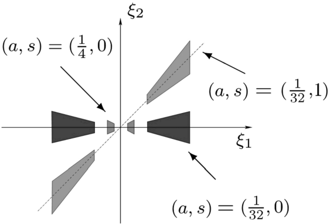
Fig. 2
Support of the classical shearlets ${\hat{\psi }_{a,s,t}}$ (in the frequency domain) for different values of a and s.
To obtain the discrete form of the continuous shearlet system and related transform, it is easy to discrete by properly sampling the scale, shear and translation parameters. A (regular) discrete shearlet system, associated with
$\psi \in {L^{2}}({R^{2}})$ and denoted by
$\mathcal{SH}(\psi )$, is defined by
which can be easily obtained by setting
$(a,s,t)=({2^{-j}},-k{2^{-j/2}},{S_{-k{2^{-j/2}}}}{A_{{2^{-j}}}}m)$. Similarly to the continuous case, the discrete shearlet transform of
$f\in {L^{2}}({R^{2}})$ is defined as the following map
where
$j,k\in Z$,
$m\in {Z^{2}}$. The main goal of utilizing shearlet systems is analysis and synthesis of 2-D data, therefore, we need to provide a discrete shearlet system
$\mathcal{SH}(\psi )$ which forms a basis or, more generally, a frame. Similar on continuous form, for each
$f\in {L^{2}}({R^{2}})$, we have the reproducing formula:
with convergence in the
${L^{2}}$ sense. Also, in Labate
et al. (
2005), Guo and Labate (
2007) it is illustrated that the classical shearlet is a well-localized function, i.e. it has rapid decay both in the spatial and in frequency domain. The well localization property of classical shearlet implies that discrete shearlet system
$\mathcal{SH}(\psi )$ forms a frame. This property is needed for obtaining optimally sparse approximations. Tiling of the frequency plane induced by discrete shearlets
${\widehat{\psi }_{j,k,m}}$ is shown in Fig.
3.
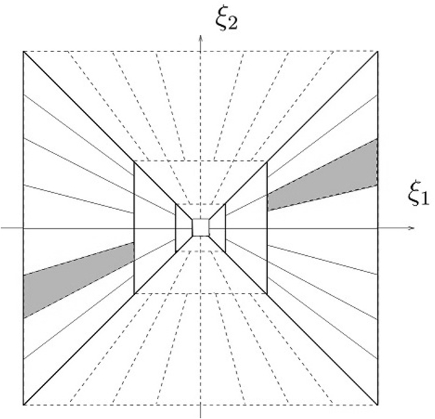
Fig. 3
Tiling of the frequency plane induced by discrete shearlets ${\widehat{\psi }_{j,k,m}}$. The horizontal region ${\mathcal{D}_{h}}$ is illustrated in solid line and the vertical region ${\mathcal{D}_{v}}$ is in dashed line.
Definition 2.
The class
${\mathcal{E}^{2}}({R^{2}})$ of cartoon-like images is the set of functions
$f:{R^{2}}\to C$ of the form
where
$B\subset {[0,1]^{2}}$ is a set with
$\partial B$ being a closed
${C^{2}}$-curve with bounded curvature,
${\mathbf{1}_{B}}(x)=\Big\{\begin{array}{l@{\hskip4.0pt}l}1,\hspace{2.5pt}\hspace{2.5pt}& x\in B\\ {} 0,\hspace{2.5pt}\hspace{2.5pt}& x\notin B\end{array}$ is indicator function and
${f_{i}}\in {C^{2}}({R^{2}})$ are functions with supp
${f_{i}}\in {[0,1]^{2}}$ and
$\| {f_{i}}{\| _{{C^{2}}}}=1$ for each
$i=0,1$.
The property of optimally sparse approximations of multivariate functions is one of the main motivations to propose the shearlet framework. Before stating the main results, we briefly describe how shearlet expansions are able to achieve optimally sparse approximations. Consider a cartoon-like function
f and let
${\mathcal{SH}_{\psi }}$ be a discrete shearlet system of (
10). For
$j\in Z$, the elements of
${\mathcal{SH}_{\psi }}$ are approximately inside a box of size
${2^{-j/2}}\times {2^{-j}}$, it follows that at scale
${2^{-j}}$ there exists about
$O({2^{j/2}})$ such waveforms whose support is tangent to the curve of discontinuity. Consequently, for
j sufficiently large, each shearlet coefficient
$\langle f,{\psi _{j,k,m}}\rangle $ can be controlled by Guo and Labate (
2007,
2012)
where
C is a constant. From inequality (
12) and the observation that there exists at most
$O({2^{j/2}})$ significant coefficients, it can be concluded that the
Mth largest shearlet coefficient is bounded by
$O({M^{3/2}})$. This implies that the following result holds.
Theorem 1.
Let $f\in {\mathcal{E}^{2}}({R^{2}})$ be a cartoon-like image defined on a bounded domain $\Omega \subset {R^{2}}$, and let ${f_{M}}$ be the approximation of f obtained by taking the M largest coefficient $|{\psi _{j,k,m}}|$ in the shearlets expansion of f given by (
11)
. Then the asymptotic approximation error is given by
Proof.
To prove see Guo and Labate (
2007,
2012) and the references therein. □
Let
${\psi _{j,k,m}}$ be a classical shearlet, according to Fig.
2, to attain the reproducing formula (
11), it is enough to compute the inner product of
$\langle f,{\psi _{j,k,m}}\rangle $ in both horizontal region
${\mathcal{D}_{h}}$ and vertical region
${\mathcal{D}_{v}}$. In Guo and Labate (
2007,
2012), for both region index
$d=\{h,v\}$, it can be shown that
where
and
${A_{h}}=\left(\begin{array}{c@{\hskip4.0pt}c}4& 0\\ {} 0& 2\end{array}\right),{S_{h}}=\left(\begin{array}{c@{\hskip4.0pt}c}1& 1\\ {} 0& 1\end{array}\right)$ and
${A_{v}}=\left(\begin{array}{c@{\hskip4.0pt}c}2& 0\\ {} 0& 4\end{array}\right)$,
${S_{v}}={S_{h}^{T}}$. In (
13), it is required to compute
$\hat{f}(\xi )$ in discrete form, so given an
$N\times N$ image
$f\in {\ell ^{2}}({Z_{N}^{2}})$, the 2D discrete Fourier transform (DFT) of
f will be:
where
$-\frac{N}{2}\leqslant {k_{1}},{k_{2}}\leqslant \frac{N}{2}$ and brackets
$[.,.]$ denote the indices of
$\hat{f}$ in Fourier domain. To compute the integrand of (
13), in the space domain and at the resolution level
j, firstly, the Laplacian-pyramid (LP) algorithm (Burt and Adelson,
1983) associated with the pseudo-polar Fourier transform (Averbuch
et al.,
2008) will be utilized. This will achieve the multiscale partition illustrated in Fig.
4, by decomposing
${f_{a}^{j-1}}[{n_{1}},{n_{2}}]$,
$0\leqslant {n_{1}},{n_{2}}\leqslant {N_{j-1}},$ into a low pass filtered image
${f_{a}^{j}}[{n_{1}},{n_{2}}],$ a quarter of the size of
${f_{a}^{j-1}}[{n_{1}},{n_{2}}],$ and a high pass filtered image
${f_{d}^{j}}[{n_{1}},{n_{2}}]$. Consequently, to compute the shearlet coefficients
$\langle f,{\psi _{j,k,m}^{d}}\rangle $ given by (
13), in the discrete domain, it is enough to compute the inverse pseudo-polar DFT and apply the inverse two-dimensional fast Fourier transform (FFT) on each decomposition level.
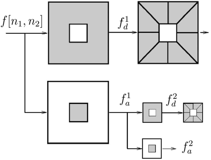
Fig. 4
The figure illustrates the succession of Laplacian-pyramid and directional filtering.
We refer to Labate
et al. (
2005), Guo and Labate (
2007,
2012) for additional information about shearlet and its applications in various sciences and engineering.
4 Non-Subsampled Shearlet Transform (NSST)
The main idea of shearlet transform is to filter signals in pseudo-polar grid (Averbuch
et al.,
2008), and then utilize a bandpass filter in frequency domain directly without sampling operations. Therefore, the directional filtering is kept away from distortion and lead to invariance in shearlet transform. Also, as described in the last section, the discrete form of shearlet transform is achieved by combination of Laplacian-pyramid (Burt and Adelson,
1983) algorithm and directional filter. To improve the computational efficiency and also to reduce the effect of Gibbs phenomena, usually the directional filter is so designed that has a small size support.
The non-subsampled form of Laplacian-pyramid filter (NSLP) is proposed by Cunha
et al. (
2006). By substituting NSLP for LP and combining it with discrete shearlet transform, non-subsampled shearlet transform (NSST) is designed to improve effectiveness of discrete shearlet transform (Hou
et al.,
2012). The NSST is known as the shift-invariant version of the shearlet transform. Since the NSST is a fully shift-invariant, multi-scale and multi-directional expansion in comparing to shearlet transform, it can diminish the effect of pseudo-Gibbs phenomena and shearlet-like artifacts in the related processing. The analysis of NSLP can be done as the following iterative processing (Hou
et al.,
2012):
where
f is an image,
${\mathit{NSLP}_{j+1}}$ is the detail coefficients at scale
$j+1$, and
$F{h_{k}^{0}}$ and
$F{h_{j}^{1}}$ are low pass and high pass filters of NSLP at scale
j and
k, respectively. Therefore, according to Fig.
4, given an
$N\times N$ image
$f\in {\ell ^{2}}({Z_{N}^{2}})$, the procedure of the non-subsampled shearlet transform associated with non-subsampled Laplacian-pyramid at a fixed resolution scale
j and in the number of direction
${D_{j}}$ can be summarized in Algorithm
1.

Algorithm 1
Non-subsampled shearlet transform
5 Proposed Algorithm and Experimental Results
In this section, firstly, we have proposed a denoising algorithm based on non-subsampled shearlet transform associated with log-transform method and secondly evaluated its performance for reducing the speckle noise of the ultrasound images. The structure of present method is similar to those described in Abazari and Lakestani (
2018a), Hou
et al. (
2012). Consider the speckle noisy problem
$u=v{n_{s}}$, where
u is observed image,
v is noise free image and
${n_{s}}$ is the multiplicative speckle noise which is independent of noise free image
v. According to relationships (
3)–(
6), after applying the log-transform, we have
where
$g=\log (u)$,
$f=\log (v)$ and
$\Upsilon =\log ({n_{s}})$. The additive noise Υ has properties similar to additive Gaussian noise. Our goal is to obtain an estimatation of
f, namely
$\tilde{f}$, from the noisy data
g by applying a classical soft thresholding scheme (Labate
et al.,
2005; Guo and Labate,
2007) on the shearlet coefficients of
g. The threshold levels are given by
${\tau _{j,k}}={c_{j}}{\sigma _{{\Upsilon _{j,k}}}},$ as in Labate
et al. (
2005), Guo and Labate (
2007,
2012,
2013), where
${\sigma _{{\Upsilon _{j,k}}}}$ is the standard deviation of noise at scale
j and shear directional band
k and
${c_{j}}$ is the scaling parameter. Here the standard deviation
${\sigma _{{\Upsilon _{j,k}}}}$ is estimated by using the MATLAB function of
std. By using Laplacian-pyramid decomposition, we used five levels of the NSLP decomposition, and we applied a directional decomposition on four of the five scales. According to Fig.
4, we used eight shear filters of size
$32\times 32$ for the first two scales (coarser scales), and sixteen shear filters of size
$16\times 16$ for the third and forth levels (fine scales) and so on. Finally, by using the exp-transformation, the estimated image can be obtained as
$\tilde{f}=\exp (\tilde{f})$. Let
f be noise free image of size
$N\times N$ and
$\tilde{f}$ denotes the estimated image, to test our algorithm and to assess its performance, we used two measurements from the following:
-
• PSNR: as peak signal-to-noise ratio, measured in decibels (dB), defined by
where
$\| .{\| _{F}}$ is the Frobenius norm.
-
• SSIM: for calculating the structural similarity (SSIM) index between denoised image
$\tilde{f}$ and original image
f, defined by Wang
et al. (
2004),
where
${\mu _{f}},{\mu _{\tilde{f}}}$ and
${\sigma _{f}^{2}},{\sigma _{\tilde{f}}^{2}}$ are the average and variance of
$f,\tilde{f}$, respectively,
${\sigma _{f\tilde{f}}}$ is the covariance of
f and
$\tilde{f}$ and
${c_{1}}={({k_{1}}L)^{2}}$,
${c_{2}}={({k_{2}}L)^{2}}$ are two variables to stabilize the division with weak denominator. Here, we set
$L=255$ as dynamic range of the pixel values and
${k_{1}}=0.01$,
${k_{2}}=0.03$.
The proposed scheme, which is briefly mentioned in Algorithm
2, is implemented using MATLAB 2012. The scours of ShearLab (
2008) are used to construct a discrete form of shearlet transform and its non-subsampled form is erected by open source files of NSCT (
2008) proposed by Minh. N. Do which initially applied for contourlet transform.
| Step 1: |
Input a speckled noisy ultrasound image u, |
| Step 2: |
Take the logarithmic transform on the speckled noisy image u to obtain f. |
| Step 3: |
Computes the discrete shearlet transform of f by applying eight shear filters of size $32\times 32$ for the first two scales (coarser scales), and sixteen shear filters of size $16\times 16$ for the third and forth levels (fine scales) and so on, associated with 5 scale, i.e. $j=1,2,\dots ,5$, see Algorithm 1. |
| Step 4: |
Compute the standard deviation ${\sigma _{{\Upsilon _{j,k}}}}$ in each scale j and shear direction k. |
| Step 5: |
Applying thresholding ${\tau _{j,k}}={c_{j}}{\sigma _{{\Upsilon _{j,k}}}}$ in the scale j and shear direction k. |
| Step 6: |
Apply the inverse discrete shearlet transform to obtain image $\tilde{f}$. |
| Step 7: |
Apply the exp-transform, $\tilde{f}:=\exp (\tilde{f})$, to obtain estimate image $\tilde{f}$. |
Algorithm 2
Proposed method
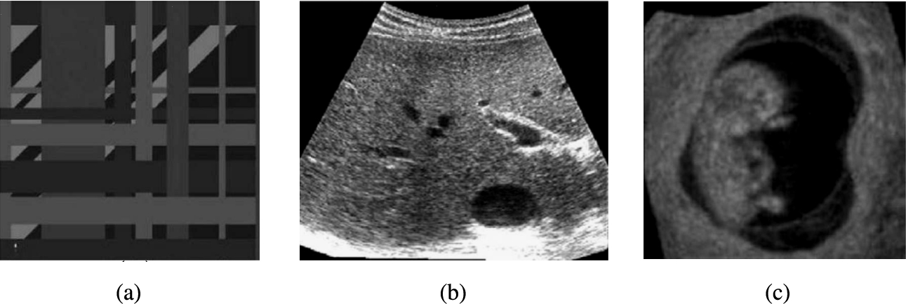
Fig. 5
Sample test images. (a) Cartoon-like image. (b) Real ultrasound image of a tumour. (c) Real ultrasound image of a fetus.
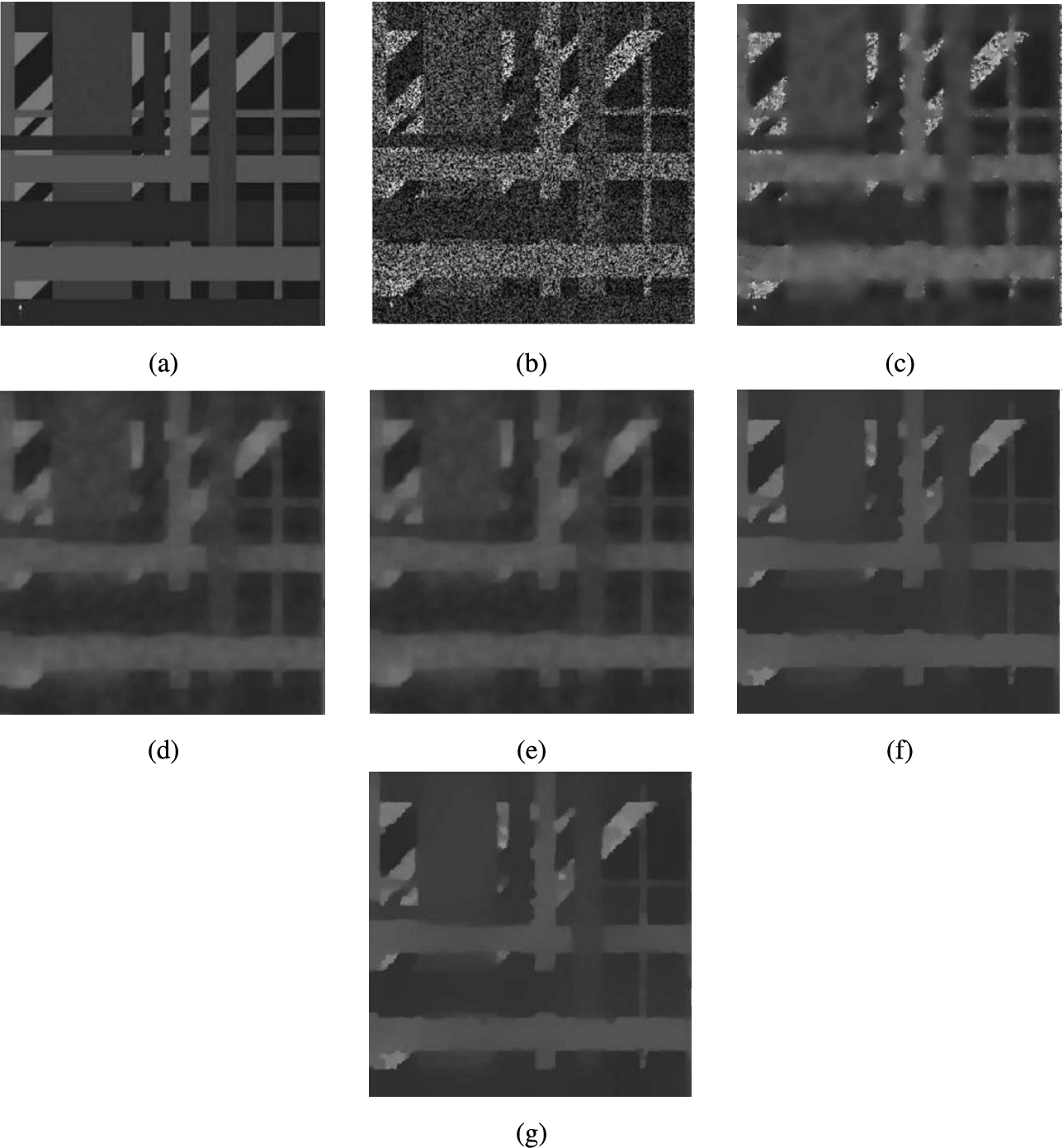
Fig. 6
Different methods of noise removal on a synthetic image. (a) Original image. (b) Image polluted by multiplicative speckle noise with Rayleigh distribution (variance is
$\upsilon =0.8$) (PSNR = 18.41, SSIM = 0.2372). (c) The denoising result using SRAD (Yu and Acton,
2002) (PSNR = 24.35, SSIM = 0.8551). (d) The result using VO method (Vese and Osher,
2003) (PSNR = 23.04, SSIM = 0.8044). (e) The denoised result using framelet regularization method without backward diffusion (Wang
et al.,
2014) (PSNR = 23.95, SSIM = 0.8164). (f) The denoised result using framelet regularization method and backward diffusion (Wang
et al.,
2014) (PSNR = 24.23, SSIM = 0.8314). (g) The result of proposed method (PSNR = 27.24, SSIM = 0.9258).
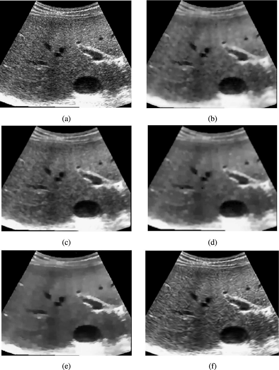
Fig. 7
Visual comparison of various speckle suppressing methods on a ultrasound image of a tumour. (a) Original image. (b) The denoising result using SRAD (Yu and Acton,
2002). (c) The result using VO method (Vese and Osher,
2003). (d) The denoised result using framelet regularization method without backward diffusion (Wang
et al.,
2014). (e) The denoised result using framelet regularization method and backward diffusion (Wang
et al.,
2014). (f) The result of the proposed method.
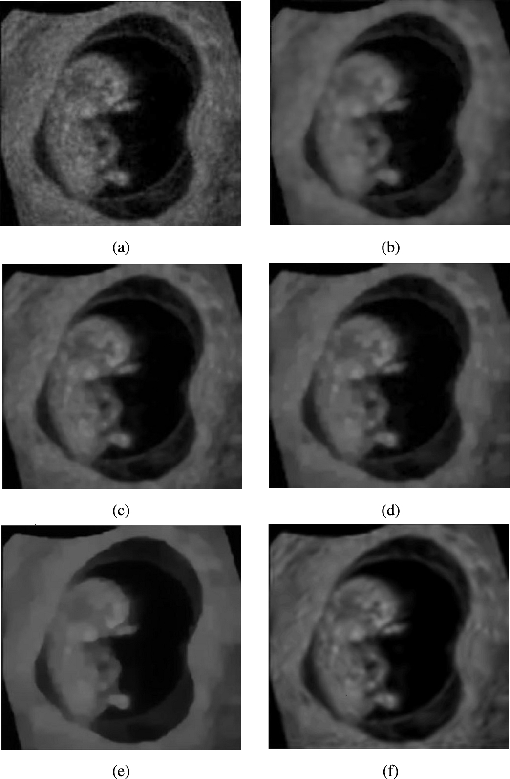
Fig. 8
Visual comparison of various speckle suppressing methods on a ultrasound image of a fetus. (a) Original image. (b) The denoising result using SRAD (Yu and Acton,
2002). (c) The result using VO method (Vese and Osher,
2003). (d) The denoised result using framelet regularization method without backward diffusion (Wang
et al.,
2014). (e) The denoised result using framelet regularization method and backward diffusion (Wang
et al.,
2014). (f) The result of the proposed method.
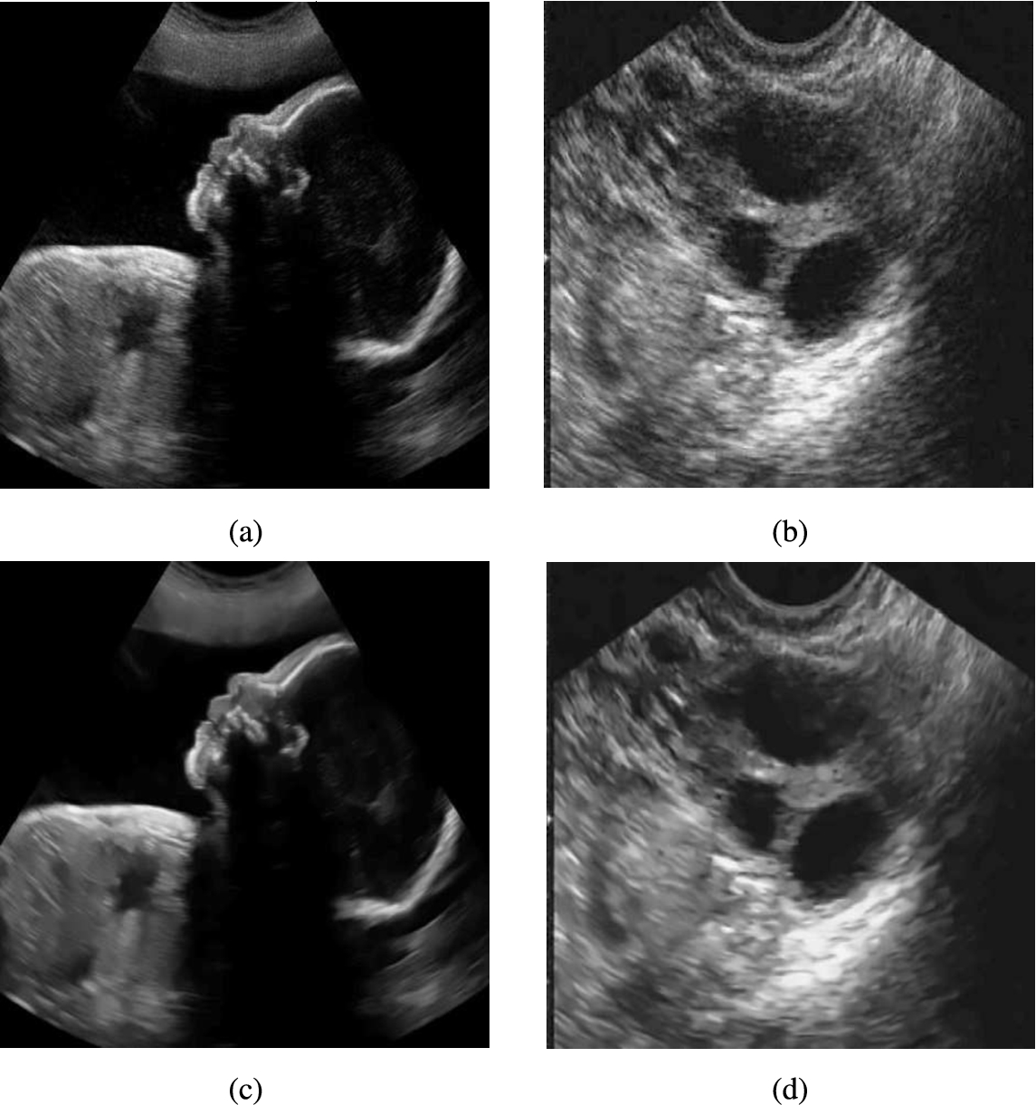
Fig. 9
Visual comparison of various speckle suppressing methods on two real ultrasound images. (a) and (b) Real ultrasound images. (c) and (d) The result of the proposed method.
In the first set, we have considered three images listed in Fig.
5 (one sample cartoon-like image and two real ultrasound images same as considered in Yu and Acton (
2002), Vese and Osher (
2003), Wang
et al. (
2014), and have compared the results of the proposed method with some related medical ultrasound despeckling techniques from the recent literature such as Yu and Acton (
2002), Vese and Osher (
2003), Wang
et al. (
2014). Firstly, we degraded a noise free sample cartoon-like image, (Fig.
5(a)), by multiplicative speckle noise with Rayleigh distribution by variance of
$\upsilon =0.8$ and then applied the proposed method on this image. To evaluate the efficiency of the proposed method, we used peak signal to noise ratio (PSNR) as a quantity to measure the quality of reconstruction of noisy images and SSIM as a structural similarity index between denoised image and original image. The despeckled image of our proposed method, (Fig.
6(g)), is compared with related techniques of Yu and Acton (
2002), Vese and Osher (
2003), Wang
et al. (
2014) with respect to PSNR and SSIM and are shown in Figs.
6(b)–
6(f). The measurements of PSNR and SSIM of the proposed method in comparison to those methods mentioned in Yu and Acton (
2002), Vese and Osher (
2003), Wang
et al. (
2014) show that the proposed approach is better than those methods, in addition, the proposed method preserves the texture and edges of images while the methods of Yu and Acton (
2002), Vese and Osher (
2003), Wang
et al. (
2014) lead to smooth edges of images. Also, to evaluate the visual quality of the proposed approach, similarly to the methods mentioned in Yu and Acton (
2002), Vese and Osher (
2003), Wang
et al. (
2014), we employed the proposed method to two real noisy medical ultrasound images (see Figs.
5(b) and
5(c) same as in Yu and Acton (
2002), Vese and Osher (
2003), Wang
et al. (
2014)). The results of our proposed method in comparison with the results of state-of-the-art methods mentioned in Yu and Acton (
2002), Vese and Osher (
2003), Wang
et al. (
2014) are listed in Figs.
7 and
8.
In the second set, two other real ultrasound images, Fig.
9(a) and
9(b), from Siemens Healthcare (Siemens Healthcare GmbH,
2019), are considered and the proposed method is applied to reduce their speckle noise. The despeckled result of these images are shown in Fig.
9(c) and
9(d), respectively, which show that our proposed method can effectively suppress the speckle noises.
Generally, experimental results of the first and the second set of selected images illustrate that the proposed approach can obtain better performance in terms of PSNR and SSIM for ultrasound image denoising. From visual comparison, it is easy to see that our proposed method gets smooth effect while preserving the edges of images, which lead to maintain the useful texture information of test images.

