Abstract
In this paper, one method for training the Support Vector Regression (SVR) machine in the complex data field is presented, which takes into account all the information of both the real and imaginary parts simultaneously. Comparing to the existing methods, it not only considers the geometric information of the complex-valued data, but also can be trained with the same amount of computation as the original SVR in the real data field. The accuracy of the proposed method is analysed by the simulation experiments. This also can be applied to the field of anti-interference for satellite navigation successfully, which shows its effectiveness in practical application.
1 Introduction
Support Vector Machine (SVM) is a high-performance machine learning algorithm, which was introduced by Vapnik in the early 1990s (Ramón and Christodoulou,
2006). SVM has been proved to have excellent performances in addressing non-linear regression problems due to the robustness against noise and interferences. In the application of SVM, there is a kind of important model that is commonly known as SVR (Ramón and Christodoulou,
2006).
The original SVR is targeted to treat real numbers. The SVRs in complex data field are also desired in some field, such as the beam forming (Ramón
et al.,
2005; Gaudes
et al.,
2007) and pattern recognition (Scholkopf and Smola,
2002; Chen and Xie,
2005). The main method for processing the complex-valued SVR model is using two separate processes for the real and imaginary parts (Bouboulis and Theodoridis,
2011) respectively, which misses the cross-information of the real and imaginary parts of a complex number.
Currently, Kernel-based methods have been employed to solve nonlinear tasks for SVRs. The key method is Reproducing Kernel Hilbert Spaces (RKHS). Wintinger’s calculus on complex RKHS was developed in dissertations (Bouboulis
et al.,
2013,
2015). It was also proved that a complex SVM/SVR task is equivalent to solving two real SVM/SVR tasks by exploiting a specific real kernel. In Bouboulis
et al. (
2012), the authors introduced how to use RHKS to solve the problem in complex data field. Different from the above-mentioned methods, we propose a model, which not only considers the geometric information of the complex-valued data, but also can be trained with the same amount of computation as the original SVR in the real data field. The proposed method also has no more additional requests for kernel function than the original SVR in real data field.
The paper is organized as follows. In Section
2, the main contributions of the paper are presented, where the model of complex SVR and the training algorithms for the model are proposed in details. In Section
3, experiments are carried out to demonstrate the performance of the proposed method, and the method is applied to anti-jamming field. Finally, the paper is concluded in Section
4.
2 Complex-Valued SVR Model
In this section, a complex SVR model and the corresponding solving algorithms are proposed. Firstly, the complex-valued original problem of SVR is introduced. Secondly, the dual problem is derived. Thirdly, Karush–Kuhn–Tucker (KKT) conditions are obtained. Finally, the solution of the original problem is achieved by solving the dual problem.
The following notations are used in this paper. The superscripts ${^{H}}$ and ${^{T}}$ denote hermitian transposition and transposition. $\| \cdot \| $ is the Euclidean vector norm. $\mathrm{Re}(.)$ and $\mathrm{Im}(.)$ denote the real and imaginary part of a complex number, respectively. $|\cdot |$ denotes modulus of a complex data. In particular, when the imaginary part of the complex data is equal to zero, $|\cdot |$ denotes absolute value.
2.1 Model Building
The real-valued SVR can be obtained by solving the following optimization problem (Ramón and Christodoulou,
2006):
Subject to the constraints
for
$i=1,2,\dots ,l$, where
$\{({x_{1}},{y_{1}}),\dots ,({x_{l}},{y_{l}})\}$ is the training set and
${x_{i}}\in {R^{n}}$,
$w\in {R^{n}}$,
${y_{i}}\in R$.
P is a penalty factor.
ε is the insensitive loss factor.
${\xi _{i}}$ and
${{\xi _{i}}^{\prime }}$ are the slack variables of the output.
P,
ε,
${\xi _{i}}$ and
${\xi ^{\prime }_{i}}$ are all real numbers. In the formula (
1), the optimal value can be obtained by finding the optimal value of its dual problem. According to the principle of real-valued SVR, an SVR model in complex field is built and the corresponding solution method is proposed. In order to simplify the expression, ‘Subject to the constraints’ will be abbreviated to ‘
$\text{s.t.}$’. The corresponding complex SVR task is formulated and expressed as
where
${x_{i}}\in {C^{n}}$,
$w\in {C^{n}}$,
${y_{i}}\in C$.
${C_{1}}$ and
${C_{2}}$ are the penalty factor of the real and imaginary parts.
ε is the insensitive loss factor.
${\xi _{i}}$ and
${{\xi _{i}}^{\prime }}$ are the slack variables in the real part of the output, and the corresponding
${\eta _{i}}$ and
${{\eta _{i}}^{\prime }}$ are in the imaginary part.
${C_{1}}$,
${C_{2}}$,
ε,
${\xi _{i}}$,
${{\xi _{i}}^{\prime }}$,
${\eta _{i}}$ and
${{\eta _{i}}^{\prime }}$ are all real numbers. The formula (
3) is a complex-valued quadratic programming problem, which also can be solved by solving its dual problem.
2.2 Dual Problem
The Lagrange function of the equation (
3) can be expressed as
where
${\alpha _{i}}$,
${\alpha _{i}^{\ast }}$,
${\beta _{i}}$,
${\beta _{i}^{\ast }}$,
${\gamma _{i}}$,
${\gamma ^{\prime }_{i}}$,
${\kappa _{i}}$ and
${\kappa ^{\prime }_{i}}$ are the Lagrange multipliers. According to the dual definition of Wolfe (Brandwood,
1983; Huang and Zhang,
2007), the partial derivatives are:
For real variables, the gradients can be obtained in the traditional way:
where
${\phi _{i}}=({\alpha _{i}}-{\alpha _{i}^{\ast }})+j({\beta _{i}}-{\beta _{i}^{\ast }})$, for all
$i=1,2,\dots ,l$. As all partial derivatives are equal to zero for saddle point conditions, the following parameters can be obtained:
for
$i=1,2,\dots ,l$. Let
${\lambda _{i}}={\alpha _{i}}-{\alpha _{i}^{\ast }}$,
${\varphi _{i}}={\beta _{i}}-{\beta _{i}^{\ast }}$, then
Accordingly to the equations (
5)–(
9), the dual problem of the equation (
4) can be solved. The solution can be presented as:
By introducing a kernel function
$K({x_{i}},{x_{j}})$:
$C\times C\to R$, the dual problem can be expressed as:
The objective function can be expressed by
${\lambda _{i}}$ and
${\varphi _{i}}$, and the formula as follows:
Assume that the optimal solution of the dual problem (
11) is
${\bar{\alpha }^{(\ast )}}={({\bar{\alpha }_{1}},{\bar{\alpha }_{{_{1}}}^{\ast }},\dots ,{\bar{\alpha }_{l}},{\bar{\alpha }_{l}^{\ast }})^{T}}$ and
${\bar{\beta }^{(\ast )}}={({\bar{\beta }_{1}},{\bar{\beta }_{{_{1}}}^{\ast }},\dots ,{\bar{\beta }_{l}},{\bar{\beta }_{l}^{\ast }})^{T}}$. The optimal solution of the primal problem can be obtained:
If the training point is support vector on the boundary, then the threshold
$\bar{b}$ can be computed:
Finally, a support vector regression function in complex data field can be obtained:
2.3 KKT Conditions
Assume that the solution of the formula (
11) is
${\bar{\alpha }^{(\ast )}}$ and
${\bar{\beta }^{(\ast )}}$, then the KKT condition of (
3) can be given in formula (
16).
for all
$i=1,2,\dots ,l$. Here, the inherent relationship among
${\alpha _{i}},{\alpha _{i}^{\ast }},{\beta _{i}}$ and
${\beta _{i}^{\ast }}$will be considered firstly.
Corollary 1.
Let ${\bar{\alpha }^{(\ast )}}$ and ${\bar{\beta }^{(\ast )}}$ be the solution of formula (
11)
, and then we have
Proof.
The proof procedure is composed of two parts.
In part 1, suppose
${\alpha _{i}}\in (0,{C_{1}})$. Based on KKT conditions in (
16), the following equations can be achieved:
By calculation of equation (
18), we have
Through combination of formulas (
16) and (
19), the following expression can be obtained:
Obviously,
${\alpha _{i}^{\ast }}=0$ can be deferred from equation (
20).
In part 2, we suppose
${\alpha _{i}}={C_{1}}$. According to KKT conditions in (
16), it is known that
${\xi _{i}}$ is an arbitrary value. And there are some cases as follows.
Part 2.1. Suppose ${\xi _{i}}=0$ and according to part 1, it is easy to get ${\alpha _{i}^{\ast }}=0$.
Part 2.2. Suppose
${\xi _{i}}\ne 0$ $({\xi _{i}}>0)$, then
By solving equation (
21),
${\alpha _{i}^{\ast }}=0$ can also be obtained.
In summary, ${\alpha _{i}^{\ast }}{\alpha _{i}}=0$ is proved to be true. With the similar method, ${\beta _{i}^{\ast }}{\beta _{i}}=0$ can be proved as well. □
According to the Corollary, we can analyse the distribution of the real and imaginary parts of the sample points on the boundary. At the same time, in order to facilitate the expression of the formula, a simple notation is introduced:
Therefore the complex domain KKT conditions can be expressed as:
The formula (
11) can be solved by using SMO (Cristianini and Shawo-Taylor,
2005; Yang and Tian,
2004) method.
2.4 SMO Algorithm
SMO algorithm is a special case of decomposing algorithm. The core of the algorithm is to update two Lagrangian multipliers corresponding to two sample points at a time, while others remain unchanged. In the complex domain, the Lagrangian multiplier variables corresponding to sample points $({x_{i}},{y_{i}})$ and $({x_{j}},{y_{j}})$ are $({\lambda _{i}},{\phi _{i}})$ and $({\lambda _{j}},{\phi _{j}})$. It is important for SMO algorithm to choose the two appropriate training points and solve the corresponding optimal problem with two Lagrangian multiplier variables. In the following, these two problems are solved.
Firstly, suppose that there are already two training points
$({x_{1}},{y_{1}})$ and
$({x_{2}},{y_{2}})$. In order to simplify the formula, let
${K_{ij}}=K({x_{i}},{x_{j}})$. Therefore the objective function (
12) can be expressed as
where
$W(\text{const})$ has no relationship with
$({x_{1}},{y_{1}})$ and
$({x_{2}},{y_{2}})$. Let the initial feasible solution of this problem is
$({\lambda _{1}^{\mathit{old}}},{\phi _{1}^{\mathit{old}}})$ and
$({\lambda _{2}^{\mathit{old}}},{\phi _{2}^{\mathit{old}}})$, and the optimal solution of the problem is the new values
$({\lambda _{1}},{\phi _{1}})$ and
$({\lambda _{2}},{\phi _{2}})$ of the two variables. In order to satisfy the constraint, the new values must satisfy
where
${s_{1}^{\mathit{old}}}$ and
${s_{2}^{\mathit{old}}}$ are constant. The formula (
25) is substituted into the objective function (
24) and takes partial derivation of
W with respect to
${\lambda _{2}}$. By simplifying, we finally get
Similarly, we can update
${\phi _{2}}$:
where
$\kappa ={k_{11}}+{k_{22}}-2{k_{12}}$ and
$\mathrm{sgn}(.)$ is signum function.
Second, we should solve the problem of selecting the two training points in the iteration. According to the definition of gradient, we choose first training point which not only violates KKT conditions but also can maximize the module of gradient.
for
$i=1,2$. Since the ultimate aim of training is to find the training points that make objective function minimize, we choose the second training point which can make greatest change of formula (
24).
3 Experimental Results
In this section, the effectiveness of the proposed method in Section
2 will be demonstrated by experiments. Then it will be applied to the anti-interference field for further verification, which is carried out by comparison of our proposed solution method with the existing Power Inversion (PI) algorithm. All the simulation experiments conducted in the paper are implemented in MATLAB.
3.1 SVR-Function Estimation
In this subsection, a regression test is performed to verify the ability of the support vector regression model to handle noise by using two function
${f_{1}}(x)={e^{jx/20}}+N$,
$x\in R$ and
${f_{2}}(x)=\frac{\sin (x)}{x}+N$,
$x\in C$. For
${f_{1}}(x)$,
$x\in [0,60]$. For
${f_{2}}(x)$,
$x={x_{r}}+$j
${x_{i}}$,
${x_{r}}$ and
${x_{i}}$ are real random variables, and
${x_{r}}\in [-4,4]$,
${x_{i}}\in [-1,1]$, j as the imaginary unit.
N is the white Gaussian noise with zero mean and variances
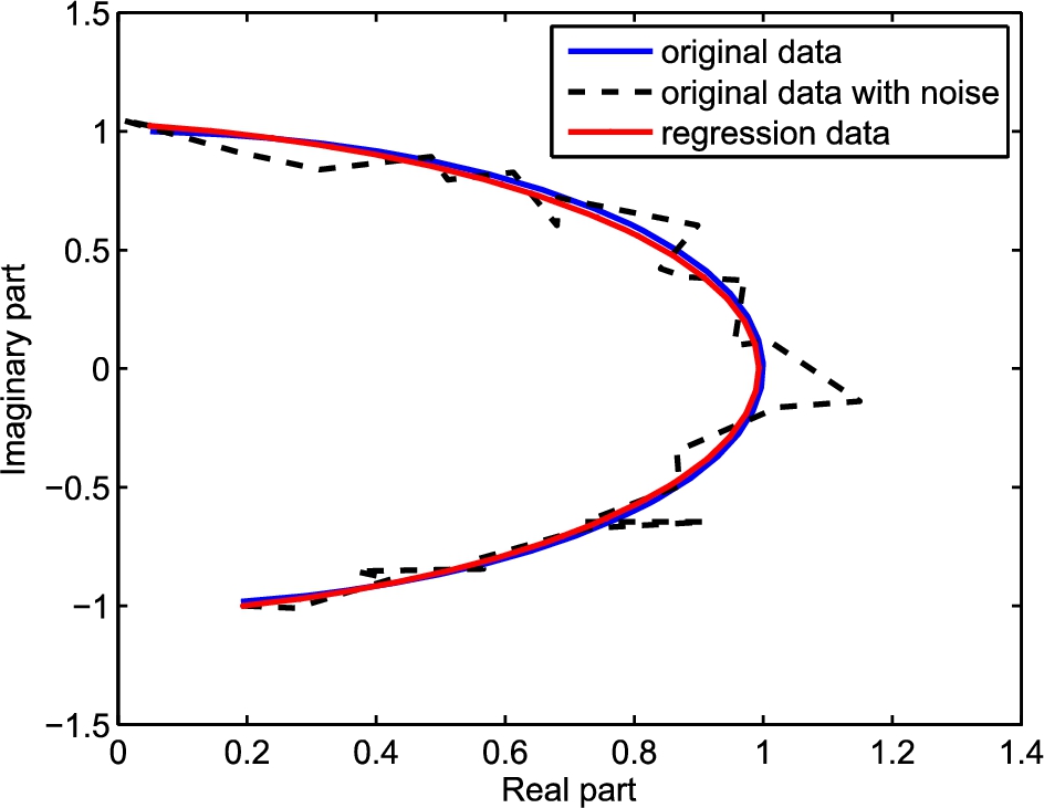
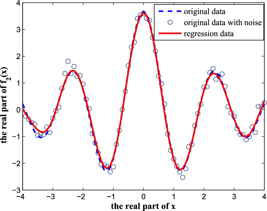
$\sigma =0.2$. The regression curves are shown in Figs.
1 and
2, which indicate that with the proposed solution method, the regression data can agree well with the original data.

Fig. 1
Regression result of ${f_{1}}(x)$.

Fig. 2
Regression result of ${f_{2}}(x)$.
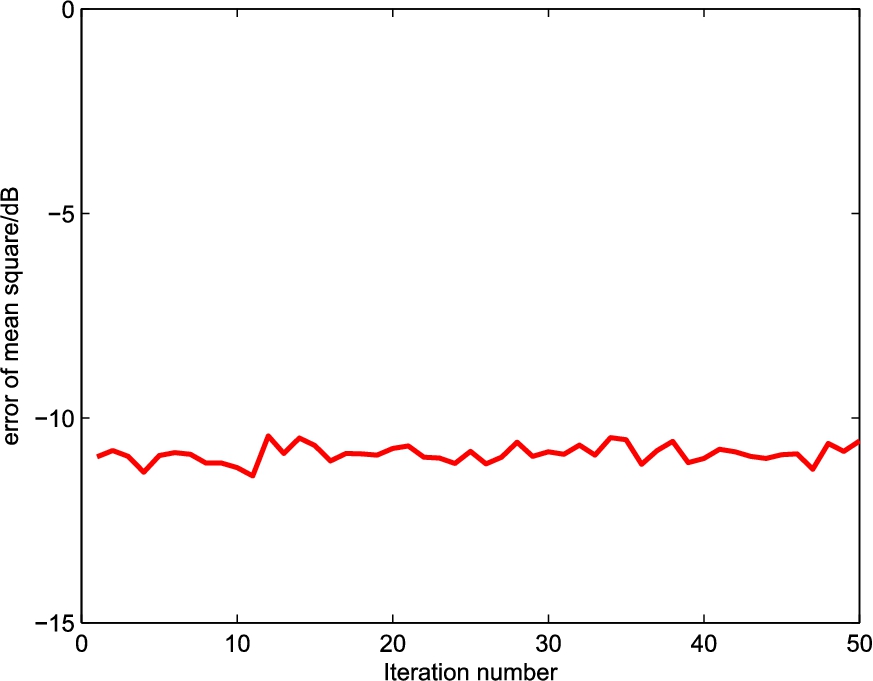
At the same time, a Monte Carlo experiment for 50 times are conducted to demonstrate the stability of the proposed solution, based on the root mean-square-error (RMSE) of complex-data defined as:
where
${\hat{x}_{t}}$ is the estimated value of
${x_{t}}$.
The resultant RMSE of the complex-data is depicted in Fig.
3, which shows that the square error is small and has a high stability.

Fig. 3
Resultant RMSE of complex-data.
In all of the above experiments, a real Gaussian Radial Basis Kernel (RBF) function is selected for SMO algorithm and the Gaussian RBF is expressed as
where
r is the Gaussian kernel parameter. For
${f_{1}}(x)$,
${C_{1}}={C_{2}}=2$,
$\varepsilon =1\text{E}-5$,
$r=50$. For
${f_{2}}(x)$,
${C_{1}}={C_{2}}=10$,
$\varepsilon =0.1$,
$r=0.8$.
Next, we compare the performance of the proposed method with CSVR (Bouboulis,
2015). The CSVR method exploits a Xcomplex kernel function and transforms the complex problem into two real SVR tasks. In order to compare the performance of the two algorithms under the same standard, the Gaussian Radial Basis kernel function is selected and
${C_{1}}={C_{2}}$. The training samples are generated by
${f_{2}}(x)$, and
${x_{r}}\in [-1,1]$,
${x_{i}}\in [-1,1]$. In this experiments,
$r=0.6$ and
$\varepsilon =0.1$ for both proposed solution and CSVR. Table
1 shows the difference in RMSE between the two algorithms under 50 Monte Carlo experiments. It can be concluded from the Table
1 that the precision of the proposed solution is roughly the same as that of CSVR.
Table 1
RMSE under different penalty factors.
| Penalty |
Proposed (RMSE) |
CSVR (RMSE) |
| ${C_{1}}={C_{2}}=2$ |
−12.89 dB |
−12.79 dB |
| ${C_{1}}={C_{2}}=10$ |
−15.17 dB |
−14.93 dB |
| ${C_{1}}={C_{2}}=20$ |
−15.23 dB |
−14.77 dB |
3.2 Application to Anti-Interference Problem
In this section, the proposed complex-SVR will be applied to the field of anti-interference to verify its effect in practical application. The anti-interference technology is an important part of array signal processing. According to the literature (Ramón and Christodoulou,
2006), the output vector of an L-element array can be described in matrix notation as:
where
S is desired signals,
J is interfere signals,
N is noise vector, and
${A_{s}}$ is the response vector of the desired signals,
${A_{j}}$ is the response vector of the interfere signals. The purpose of the anti-interference is to obtain desired output
S and suppress interfere signal. Therefore, the output of the array processor is
where
W is the weight vector of the array,
d is the estimated value of the desired signal
S,
ε is the estimation error. In practical applications, we only know the output vector of the array. Therefore, in order to achieve interference suppression, it is important to know how to use the output vector
X of an L-element array to get the optimal weight vector W.
Firstly, it is important to generate the training data. For an L-elements Unit Circular Array (UCA), a dataset
$X(k)={[{x_{1}}(k),{x_{2}}(k),\dots ,{x_{l}}(k)]^{T}}$ can be obtained, where
$1<k<N$ and
N is the snapshot number and
${x_{i}}(k)$ is the received value of the
$i-th$ element at moment
k. The autocorrelation matrix of all samples can be computed by
According to the PI algorithm (Zahm,
1973; Compton,
1979), the optimal weight is
where
$\mathrm{Const}={[1,0,\dots ,0]^{T}}$. And then a set of pairs
$\{R,W\}$ can be chosen as training samples.

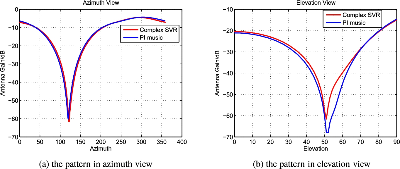
Fig. 4
The arrays pattern of the original PI algorithm and complex SVR.
Secondly, we will show how to use Complex-SVR to achieve anti-interference. The narrowband signal is chosen as the jammer, whose direction is
$\theta ={120^{0}}$,
$\varphi ={50^{0}}$, where
θ is the azimuth,
φ is the elevation angle. In this experiment, a 4-element UCA is chosen and the data
X is divided into 100 sections (where
$N=12800$), so as to have 128 snapshots in each section. Then, based on the equations (
34) and (
35), 100 sample data can be obtained. In the experiment, 70 sample data are chosen as training samples, and the remaining 30 points as the testing samples. In this experiment,
${C_{1}}={C_{2}}=20$,
$\varepsilon =1\mathrm{E}-4$,
$r=0.8$. The arrays patterns of PI and the proposed complex-valued SVR are illustrated in Fig.
4. where Fig.
4(a) is a pattern of the azimuth angle when the elevation angle is fixed. and Fig.
4(b) is a pattern of the elevation angle when the azimuth angle is fixed. The antenna gain is defined as
It can be seen from Fig.
4 that complex-valued SVR can get deeper nulls in the direction of the interfering signals than PI.
4 Conclusion
A complex-valued model of SVR was proposed in the paper. The proposed method considers all the information of both the real and imaginary parts of the SVR model. Compared to conventional SVR model, the great feature is that although the method has both the real and imaginary parts information, it does not require extra amount of computation. The accuracy and stability of the proposed model of SVR are finally demonstrated by experiments. In addition, it was also applied to the anti-interference of satellite navigation system for verification of its effect in reality. The results indicate that the proposed method achieved much better performance the normal PI algorithm.
Acknowledgements
The authors would like to thank the editor and referees for their valuable suggestions and comments. Yongtang Shi is partially supported by the Natural Science Foundation of Tianjin (No. 17JCQNJC00300) and The National Natural Science Foundation of China.
References
Bouboulis, P. (2015). Complex soupport vector machines for regression and quaternary classification. IEEE Transaction on Neural Networks and Learning Systems, 26(6), 1260–1274.
Bouboulis, P., Theodoridis, S. (2011). Extension of Wirtinger’s calculus to reproducing kernel Hilbert spaces and the complex kernel LMS. IEEE Transactions on Signal Processing, 59(3), 964–978.
Bouboulis, P., Theodoridis, S., Mavroforakis, C. (2012). Complex support vector regression. In: IEEE Conference Publications, pp. 1–6.
Bouboulis, P., Theodoridou, E., Theodoridis, S. (2013). Complex support vector machines for quaternary classification. In: IEEE International Workshop on Machine Learning for Signal Processing, Southcamption, UK, pp. 22–25.
Bouboulis, P., Theodoridis, S., Mavroforakis, C., Evaggelatou-Dalla, L. (2015). Complex support vector machines for regression and quaternary classification. IEEE Transcation on Neural Networks and Learning Systems, 26(6), 1260–1274.
Brandwood, D.H. (1983). A Complex gradient operator and its application in adaptive array theroy. IEE Proceedings F – Communications, Radar and Signal Processing, 130, 11–16.
Chen, G.Y., Xie, W.F. (2005). Pattern recognition using dual-tree complex wavelets features and SVM. In: IEEE Conference Publications, Saskatoon, pp. 2053–2056.
Compton, R.J. (1979). The power-inversion adaptive array–concept and performance. IEEE Transaction on Aerospace and Electronic Systems, 15(6), 803–814.
Cristianini, N., Shawo-Taylor, J. (2005). Support Vector Machines and Other Kernel-Based Learning Methods. China Machine Press.
Gaudes, C.C., Santamaria, I., Via, J., Gomez, E.M., Paules, T.S. (2007). Robust array beamforming with sidelobe control using support vector machines. IEEE Transactions on Signal Processing, 55(2), 574–584.
Huang, Y., Zhang, S. (2007). Complex matrix decomposition and quadratic programming. Mathematics of Operations Research, 32(3), 758–768.
Ramón, M.M., Christodoulou, C. (2006). Support Vector Machines for Antenna Array Processing and Electromagnetics. Morgan & Claypool Publishers.
Ramón, M.M., Xu, N., Christodoulou, C.G. (2005). Beamforming using support vector machines. IEEE Antennas and Wireless Propagation Letters, 4(1), 439–442.
Scholkopf, B., Smola, A. (2002). Learning with Kernels: Support Vector Machines, Regularization, Optimization and Beyond. MIT Press, Cambridge, MA, USA.
Yang, D., Tian, Y. (2004). A New Method of Data Mining-Support Vector Machine. Science Press, Beijing.
Zahm, C.L. (1973). Application of adaptive arrays to suppress strong jammers in the presence of weak signals. IEEE Transaction on Aerospace and Electronic Systems, 9(3), 260–271.

