1 Introduction
Image processing incorporates a variety of manipulations designed in order to provide desired information or specific image quality that is application depended. Although both optical and analog image processing have a great importance in the image acquisition processes, digital image processing has a dominant role in a number of applications such as intelligent watermarking, video telephony or pattern recognition. With high-growing market, these applications became very important and high quality of images is required. The final objective is to achieve as high as possible image quality at the given bit-rate. On the other hand, age of information sets new hardware requirements with the rapid growing, setting limited data storage, low processing delay or hardware simplicity as important demands. As a result, digital image compression has a key role in development of future systems.
Block truncation coding (BTC) is the image compression method proposed by Delp and Mitchell (
1979). Its quite simple design and capability to introduce other various techniques into the algorithm made it very popular and a common tool for solving different problems. Currently, it is commonly used to compress a video to be stored in frame memory for display devices such as LCDs (Kim
et al.,
2016) and it is widely used for LCD overdrives (Kim and Lee,
2016). Furthermore, modern watermarking techniques are very often based on block truncation coding – in Chang
et al. (
2015) it is proposed high capacity reversible data hiding scheme based on residual histogram shifting for compressed images of block truncation coding whereas high capacity data hiding scheme for error-diffused block truncation coding is presented by Guo and Liu (
2012). Next, SVD-based tamper detection and self-recovery algorithm using active watermarking and block partitioning is discussed in Dadkhah
et al. (
2014). Moreover, BTC method can be successfully applied to the systems that deal with both grayscale and colour images (Lema and Mitchell,
1984; Chang
et al.,
2008).
Also, colour image quantization has been researched in recent years and some methods based on artificial bee colony algorithm (Ozturk
et al.,
2014) or designed for specific feature extraction (Ponti
et al.,
2016) were proposed. Besides that, current problems require application of various techniques to biometric systems, pattern recognition, computer vision or medical imaging making the image processing algorithms research very important (Barcellos
et al.,
2015; Alomari
et al.,
2016). In this paper, we are focused on piecewise-uniform quantizer designing and its application to the algorithm which processes grayscale images.
Issues that originate during image acquisition and image-processing steps that were applied to the image during digital image processing, such as those involving contrast and dynamic range mismatch, can be successfully depicted using a histogram (Salomon,
2007). Histograms are frequently used to determine whether an image is making effective use of its intensity range by analysing the size, shape and form of the histogram’s distribution. In Savic
et al. (
2012) a model for
PSQNR (peak signal-to-quantization-noise ratio) calculation which exploits weighting function for averaging was presented. However, this function depends on the input dataset and closed-form solutions are not provided. In this paper, we will consider a histogram of variances which is focused on distinction between a pixel value and a mean value of all pixels in a block that the pixel belongs to. This kind of histogram will be researched in order to make an analytical model with closed-form solutions for performance estimation of the proposed system. Besides
PSQNR, estimation of the total average bit-rate will be provided due to a great influence of applied Golomb–Rice coding as a lossless data compression method (Perić
et al.,
2010a,
2010b). The histogram will be modelled by introducing Inverse Gaussian function in order to provide general closed-form solutions.
Besides providing a novel analytical model, emphasize of the paper is to propose an improved quantizer design, in order to improve overall system performance of block truncation coding. Improvements are done by applying Golomb–Rice binary coding of the piecewise uniform quantizer’s output signal as well as by determining its optimal support range, discussing the influence of the discrete designing variance. Variable-length coding is already presented in both software and hardware solutions in a number of schemes that are exploited in image processing techniques, including the state-of-the-art solutions (Sayood,
2006; Salomon,
2007). JPEG-LS exploits various schemes for adaptive coding of residuals such as arithmetic coding and the Merhav–Seroussi–Weinberger scheme (Ali and Manzur,
2015). Moreover, some hardware solutions are already proposed, making Golomb–Rice coding suitable for both software and hardware applications (Kim
et al.,
2011). Next, hybrid model for compression of Laplacian source, discussed in Perić
et al. (
2010a), exploits Golomb–Rice output levels coding. However, the authors discussed hybrid model only for the unit variance, which is not suitable for image compression applications. Furthermore, aforementioned hybrid quantizer deals with continual signals whereas image compression system that we discuss considers discrete signals. In this paper, we propose Golomb–Rice coding application for designing core quantizer encoders, such as those applied in block truncation coding, and we discuss its performance for medium bit-rates that provide very high image quality. The obtained closed-form solutions depend on the input signal variance as well as discrete designing variance. Furthermore, this way designed quantizer encoder can be applied also in the other different and more complex image processing algorithms. In the end, it will be shown that this way improved simple block truncation coding system outperforms other similar techniques that incorporate linear prediction (Savic
et al.,
2015) and forward edge-based adaptation (Mathews and Nair,
2015). The system which incorporates linear prediction of the neighbouring pixel values (Savic
et al.,
2015), exploits advantages of both uniform and piecewise uniform quantizers to perform additional data transfer in order to improve previously predicted values. However, this way applied dual-mode quantization is performed only on about 70% of the pixels, as the prediction provides satisfactory results at 30% of blocks (size
$4\times 4$). However, we have to note that even though the proposed quantizer design provides high image quality, few existing techniques that incorporate vector instead of scalar quantization (Simic
et al.,
2017) or transformation coding, such as wavelet or curvelet (Li
et al.,
2010,
2013), provide higher compression ratio but also demand higher processing delay and have significantly higher complexity.
The paper is organized as follows. Section
2 describes the proposed coding algorithm and piecewise uniform quantizer design with Golomb–Rice coding. Next, Section
3 proposes a novel analytical model with closed-form solutions, based on Inverse Gaussian function introduction. Finally, experimental results and comparison with other similar models are shown in Section
4.
2 Coding Algorithm and Piecewise Uniform Quantization
In the case when it is necessary to operate with discrete data, quantization process is very often done in two steps. The first one deals with the received continual signal where continual samples have to be quantized with the fixed uniform quantizer
${Q_{0}}$, described with
${N_{0}}$ quantization levels. This way obtained samples,
$X=\{{x_{1}},{x_{2}},\dots ,{x_{{N_{0}}}}\}$, are further quantized with quantizer
${Q_{1}}$ in order to perform additional data compression. Usually, quantizer
${Q_{0}}$ performs quantization with the high number of quantization levels. For grayscale images
${N_{0}}=512$ since that block truncation coding algorithm is based on quantization of distinction between a pixel value and the mean value of all pixels in a block that pixel belongs to, where
${x_{1}}=-255$ and
${x_{{N_{0}}}}=255$ (pixels of an image can take integer values from 0 to 255). On the other hand, quantizer
${Q_{1}}$ should deal with a low or medium number of quantization levels, in order to make a compromise between reconstruction quality and the total average bit-rate. Nowadays, algorithms that discuss low number of quantization levels, providing lower image quality, are much more researched (Simic
et al.,
2017). Thus, in this paper we will discuss piecewise uniform quantizer
${Q_{1}}$ with
$N=16$ and
$N=32$ quantization levels, i.e. with medium number of levels.
It is well-known from literature that Laplacian information source provides excellent modelling of distinction between pixel value and the mean value of all pixels in a block, i.e. provides satisfactory matching between block truncation coding algorithm and reality (Jayant and Noll,
1984). Consequently, we will suppose that information source has Laplacian distribution with a memoryless property and mean value equal to zero. It is defined with:
The second step of quantization process provides quantization of discrete output samples from quantizer
${Q_{0}}$ by using
N quantization levels, where
$N<{N_{0}}$, providing additional data compression. Probabilities of these discrete input levels, considering Laplacian source, are defined with:
Design of the piecewise uniform quantizer
${Q_{1}}$ will be done as follows. Firstly, a piecewise uniform quantizer for the unit variance is designed. Its threshold values are obtained by using optimal compandor, whose compressor function is defined by Jayant and Noll (
1984):
where
${t_{\max }}$ denotes maximal signal amplitude. Boundaries between segments can be calculated with:
In previous expressions,
${t_{\max }^{\sigma =1}}$ represents the optimal maximal signal amplitude for the unit variance and its values are taken from (Perić
et al.,
2009). The value depends on the number of quantization levels –
${t_{\max }^{\sigma =1}}=6.01$ for
$N=16$ and
${t_{\max }^{\sigma =1}}=7.91$ for
$N=32$. Furthermore, the number of uniform output levels in each segment is denoted with
M and it can be calculated as
$M=N/L$.
The width of each region cell within a segment is equal to:
Furthermore, decision thresholds of the piecewise uniform quantizer, designed for the unit variance, can be obtained as:
Finally, the output levels are defined with:
In Eqs. (
4)–(
8)
i denotes a segment while
j denotes the output level within the observed segment. Due to the fact that compressor function
$c(x)$, defined with Eq. (
3), maps the input range to
$(-{t_{\max }},{t_{\max }})$ wherein
${t_{\max }^{\sigma =1}}\ll {x_{{N_{0}}}}$, denormalization will be done by using a discrete designing variance
$\hat{\sigma }$ as follows:
Finally, quantization levels could be written in a simpler form using one index, as:
where index
k, that corresponds to indices
i and
j, is obtained as
$k=(i-1)M+j$.
2.1 Golomb–Rice Coding
After quantization with
${Q_{0}}$ and
${Q_{1}}$, signal is encoded with a binary Golomb–Rice encoder at the output of designed quantizer encoder. In order to apply Golomb–Rice code described with parameter
$m={2^{k}}$,
N quantization levels have to be divided into
S segments. Taking into account symmetry of the quantizer
${Q_{1}}$, we will consider that
$S=L/2$, i.e.
S is equal to the number of segments in the positive range of quantizer
${Q_{1}}$, in order to simplify encoding design. This way, each Golomb–Rice segment will cover the corresponding symmetric ranges from the quantizer
${Q_{1}}$ in both positive and negative range. Segments are indexed with
$0,1,\dots ,S-1$. The total number of quantization levels has to be equal to:
When organizing encoding process in this way, it can be seen that
m represents the number of output levels in each segment of variable length coding. Finally, the codeword of the
jth segment (
$0\leqslant j\leqslant S-1$) is formed as
$\underset{j}{\underbrace{XX}}0\underset{k}{\underbrace{x\dots x}}$ and its length is (Perić
et al.,
2010a):
2.2 Algorithm for Image Processing
In this section, we will explain the application of the previously described quantizer on grayscale image processing. The algorithm is performed from left to right and from top to bottom and it consists of the following steps:
-
1. The image is divided into a set of non-overlapping blocks, whose size is $n\times n$ (we will use $n=4$). Each block is processed separately.
-
2. The average pixel value
${x_{\mathrm{av}}}$ of the block is found. Next, this value is quantized (with uniform quantizers using 6 bits) and obtained quantized average value
${\hat{x}_{\mathrm{av}}}$ is transmitted to the receiver (Savic
et al.,
2010).
-
3. The difference block of size
$n\times n$ is formed. Its elements are obtained as the difference of the pixel values of the current block
${x_{i,j}}$ and its quantized mean value
${\hat{x}_{\mathrm{av}}}$, and they are denoted with
${d_{i,j}}$,
$i=1,\dots ,n$;
$j=1,\dots ,n$:
-
4. Quantization of elements ${d_{i,j}}$ is done using the proposed quantizer ${Q_{1}}$.
-
5. Quantized elements denoted with ${\hat{d}_{i,j}}$ are binary coded with Golomb–Rice code and transmitted to the receiver.
-
6. In the receiver, after the reception of
${\hat{x}_{\mathrm{av}}}$ and
${\hat{d}_{i,j}}$, the reconstruction of all pixels of the original image is done as:
-
7. Go to the step 2 until all blocks are processed.
3 Analytical Model for Performance Analysis
Besides analysis of the piecewise uniform quantizer design and its optimization, the main goal of this paper is to propose a novel analytical model for grayscale image compression performance estimation. The model considers the proposed quantizer design and modified block truncation coding algorithm described in Section
2.2 and it is based on a modelling of histogram of variances whereas distinction between a pixel and the mean pixel value of all pixels in a block that pixel belongs to, is considered as the input signal. The aforementioned histogram is obtained by processing ten standard test grayscale images (Baboon, Bridge, Couple, Jet, Cart, Lena, Pepper, Ship, Street and Church).
In order to analyse and make a model of such histogram, we have researched various distributions such as Rayleigh, Lognormal, Birnbaum-Saunders and Laplacian. However, the best results we have achieved were by using general Inverse Gaussian distribution that is defined with:
Its support range is
$x\in (0,+\infty )$ whereas the mean parameter is (
$\mu >0$) and
λ is the shape parameter
$(\lambda >0)$. The parameters of Inverse Gaussian distribution are estimated by using maximum likelihood estimation method (MLE) which represents one of the standard methods and probably the most versatile one. However, the parameters could be estimated also by using other methods such as method of moments or least squares estimation method. If we suppose that
${x_{1}},{x_{2}},\dots ,{x_{n}}$ are independent and identically distributed observations, likelihood function is defined with:
where
θ is a vector of parameters. After substituting Eq. (
16) in Eq. (
17), likelihood function for Inverse Gaussian distribution is obtained:
Finally, assuming that the log-likelihood function
$\log (L(\mu ,\lambda ))$ is differentiable, unknown parameters are estimated as:
In order to transform Inverse Gaussian function to a probability density function (Fig.
1), unknown parameters will be estimated analogously to Eq. (
19) and Eq. (
20) as:
where
g represents the number of considered discrete variances of the input signal
${\sigma _{i}}$ whereas
$h({\sigma _{i}})$ represents weighting function of the observed set of images. In the end, we have obtained
$\hat{\mu }=11$ and
$\hat{\lambda }=8.4$ for such set of test images by using described method. Figure
1 shows both histogram of variances and corresponding Inverse Gaussian model for parameters calculated using Eqs. (
21)–(
22).
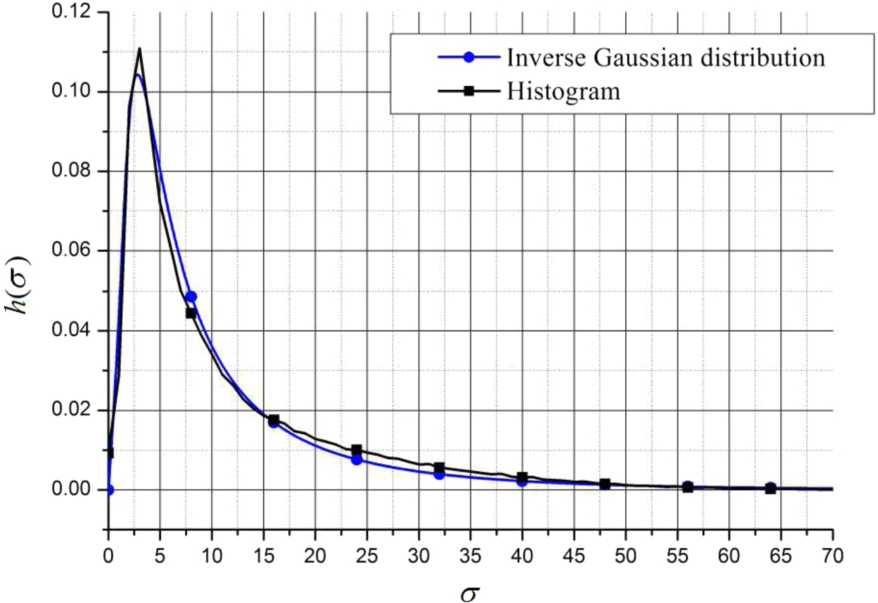
Fig. 1
Histogram of variances and Inverse Gaussian model.
In order to calculate the total average bit-rate of the proposed image compression algorithm, we propose two models. The first one is more precise and it is based on the proposed piecewise uniform quantizer design (M1 model) – all discrete thresholds and quantization levels are exploited in the same way as for PSQNR calculation. The other model is based on the optimal companding technique and it includes some additional error, but the obtained analytical expressions are much simpler and it is not necessary to memorize thresholds and quantization levels values (M2 model).
M1 model uses piecewise uniform quantizer with compressor function described with Eq. (
3) while Golomb–Rice coding is performed as it was described in Section
2.1. Since that Laplacian source is considered at the entrance, compressor function can be defined as:
The input signal will be coded using codewords of length
${l_{j}}$ (Eq. (
13)) with probabilities:
In Eqs. (
24)–(
26) and Eqs. (
30)–(
32) with
${d_{i}}$ (
$1\leqslant i\leqslant S-1$) are denoted discrete threshold values and it is valid
${d_{i}}(\hat{\sigma })={\omega _{i-1,M}}$, whereas
${d_{S}}=255$. Furthermore,
$p(x)$ is Laplacian distribution defined with Eq. (
1). Finally, the average bit-rate for the single variance is calculated with:
where
σ represents the variance of distinction between a pixel value and mean value of all pixels in a block that pixel belongs to and it represents the input signal of the quantizer. Figure
2 shows the total average bit-rate dependence on the input signal variance. By observing Fig.
2, it can be clearly seen that the average bit-rate is strongly dependent on the input signal variance. Consequently, for considering the wider set of signals, the weighting function has to be included. As a result, the total average bit-rate of the model M1 is obtained by using weighting function for averaging and taking into account the required number of bits for transmitting
${x_{\mathrm{av}}}$ (Section
2.2) as:
In previous equation, probabilities of segments
${P_{j}}({\sigma _{i}},\hat{\sigma })$ are defined with Eqs. (
24)–(
26) where thresholds are obtained using compressor function from Eq. (
23). Moreover,
${r_{\mathrm{av}}}$ denotes the required number of bits for transmitting
${x_{\mathrm{av}}}$ and it is equal to 0.375 [bpp]. For comparison, instead of
$w({\sigma _{i}})$ which represents Inverse Gaussian distribution, it will be used
$h({\sigma _{i}})$, i.e. original histogram. The same averaging will be performed in both Eq. (
33) and Eq. (
35) in order to obtain the total average bit-rate and
PSQNR of the M2 model, respectively.
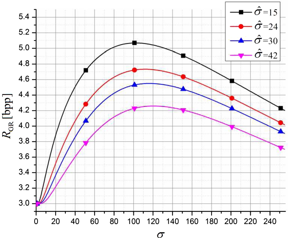
Fig. 2
${R_{\mathrm{GR}}}$ dependence on the input signal variance for various values of $\hat{\sigma }$ (M1 model).
The second model (M2) is based on the optimal companding quantizer application. The compressor function of such quantizer is defined with:
Probabilities of segments defined with Eq. (
29) are:
Finally, the total average bit-rate of the model M2 is obtained by using weighting function for averaging and taking into account the required number of bits
${r_{\mathrm{av}}}$ for transmitting
${x_{\mathrm{av}}}$ (Section
2.2) as:
In Eq. (
33), unlike Eq. (
28) probabilities of segments
${P_{j}}({\sigma _{i}},\hat{\sigma })$ are defined with Eqs. (
30)–(
32) where thresholds are obtained using compressor function from Eq. (
29).
Because of the fact that the proposed model describes a kind of a lossy image compression method, some information will be lost irreversibly during the quantization process. In order to measure reconstructed signal quality, we estimate distortion (
D) that represents a standard measure. It can be calculated with Savic
et al. (
2012):
where
${t_{k,j}}\in {Z_{k}}$ are input levels for which the quantization level is
${y_{k}}$, whereas parameter
${q_{k}}$ denotes the number of input levels mapped with
${y_{k}}$, where
${\textstyle\sum _{k=1}^{N/2}}{q_{k}}={N_{0}}/2$.
${Z_{k}}$ are non-overlapping and non-negative subsets of the set
X where
${Z_{k}}=\{{x_{k1}},\dots ,{x_{k{q_{k}}}}\}$ and
${\textstyle\bigcup _{k=1}^{N/2}}{Z_{k}}={X^{+}}$, whereas with
${X^{+}}$ is denoted the subset which consists of all non-negative elements of the set
X. Furthermore, probabilities of discrete input levels are defined with Eq. (
2). Finally, taking previous consideration into account, including weighting averaging for observed test grayscale images, reconstructed image quality calculated by using the proposed analytical model will be denoted with
${\mathit{PSQNR}_{\mathrm{wav}}}$. This measure will be calculated as:
where
In previous equation
${x_{\max }}$ represents the maximal theoretical pixel value of an image (for grayscale images
${x_{\max }}=255$).
4 Numerical Results and Discussion
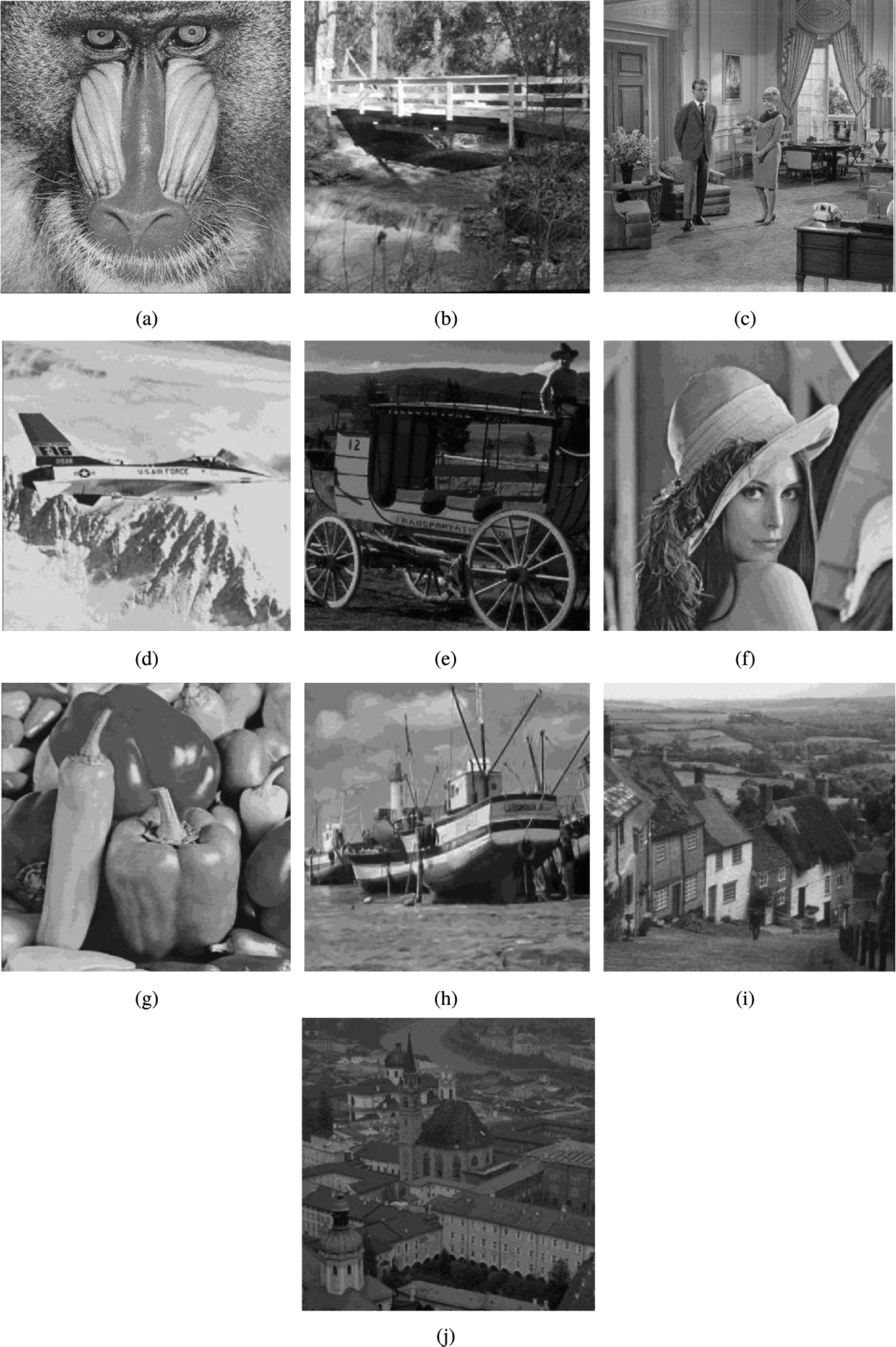
Fig. 3
Standard test grayscale images: (a) Baboon; (b) Bridge; (c) Couple; (d) Jet; (e) Cart; (f) Lena; (g) Pepper; (h) Ship; (i) Street; (j) Church.
This section provides experimental results of applying the proposed design and comparison with the results obtained by using described analytical model, as well as comparison with the other algorithms. The experiments are done for the set of ten standard test grayscale images (Baboon, Bridge, Couple, Jet, Cart, Lena, Pepper, Ship, Street and Church) of resolution
$n\times n$ pixels
$(n=512)$. These ten images are shown in Fig.
3. Unlike theoretical calculations, experimentally measured reconstructed image quality using
PSQNR can be obtained as:
where
MSE is mean squared error between original and reconstructed images and it is defined with:
where summation is done for all pixels of an image.
First of all, we provide a detailed analysis for the case when the number of quantization levels is $N=16$ and the number of segments is $L=8$. This case is chosen since it has low complexity and Golomb–Rice coding has great influence $(k=2)$ that will be discussed later.
Figure
4 shows theoretical comparison of
PSQNR values, obtained by using the exact histogram of variances and the proposed closed-form solutions based on Inverse Gaussian distribution.
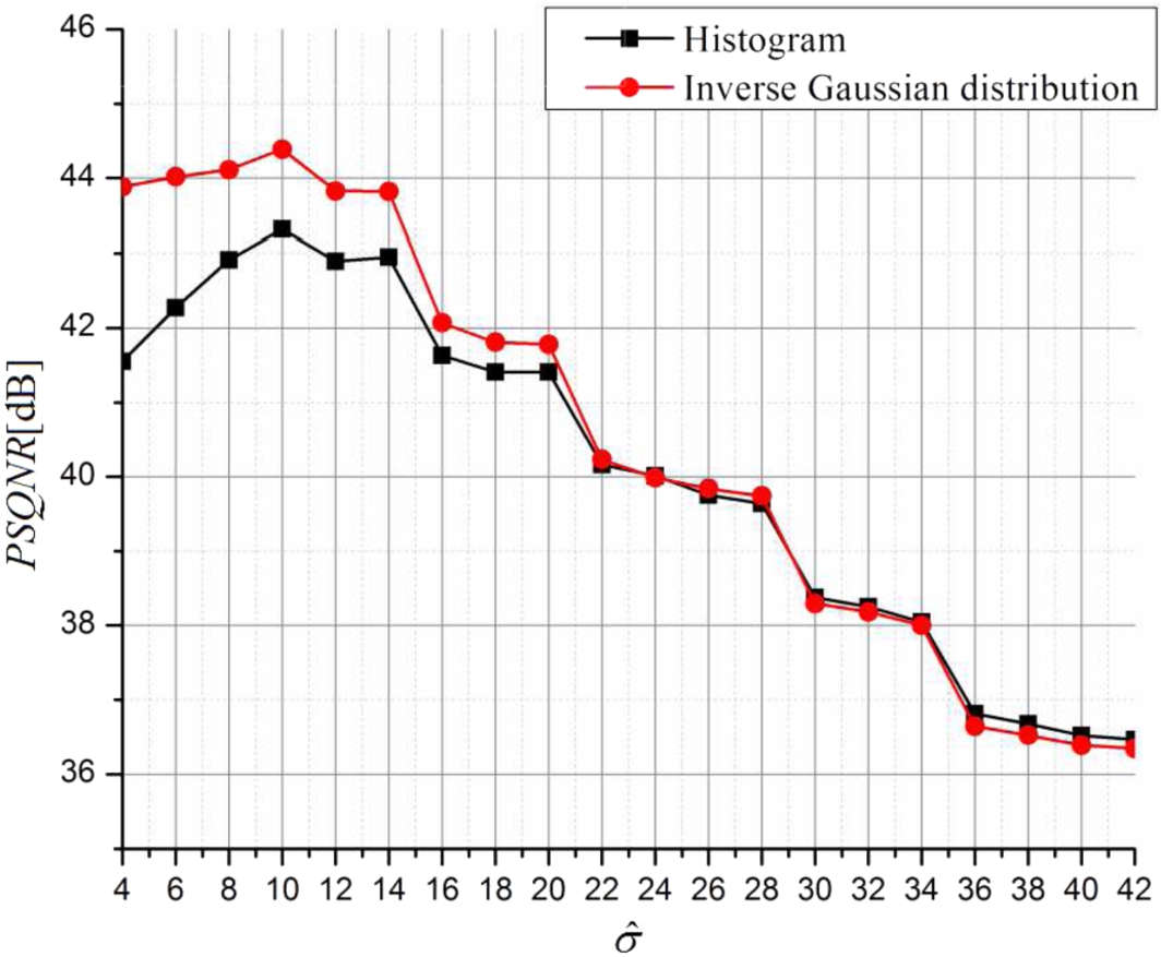
Fig. 4
PSQNR – analytical model.
By observing Fig.
4, it can be seen that with increasing the value of discrete designing variance
$\hat{\sigma }$, matching between the proposed closed-form solutions and analytical model that exploits the exact histogram is getting better and almost equal. However, a mismatch that can be noticed occurs due to variance mismatch within two quantization steps (Perić
et al.,
2015) as well as it occurs to a non-ideal modelling using Inverse Gaussian distribution for low variances. Finally, the highest
PSQNR is provided for such value of
$\hat{\sigma }$ that is almost equal to the corresponding mean value of the modelled input signal (
$\hat{\mu }=11$), justifying the term “designing variance” for parameter
$\hat{\sigma }$ (Perić
et al.,
2015).
By applying Eq. (
28) and Eq. (
33) for the observed case (
$N=16$,
$L=8$), we have obtained theoretical values for the total average bit-rate. These results are shown in Fig.
5, and the performance of the proposed analytical model is compared with the values obtained by using the exact histogram values. By observing Fig.
5, it can be seen that the proposed closed-form expressions achieve great matching with the corresponding values obtained by using the exact histogram. Also, it can be noticed that the values obtained by using piecewise uniform quantizer for calculations (M1 model) predict higher bit-rates in comparison to the corresponding values obtained by using optimal compandor (M2 model). Later, Table
1 will show that M1 model is more precise.
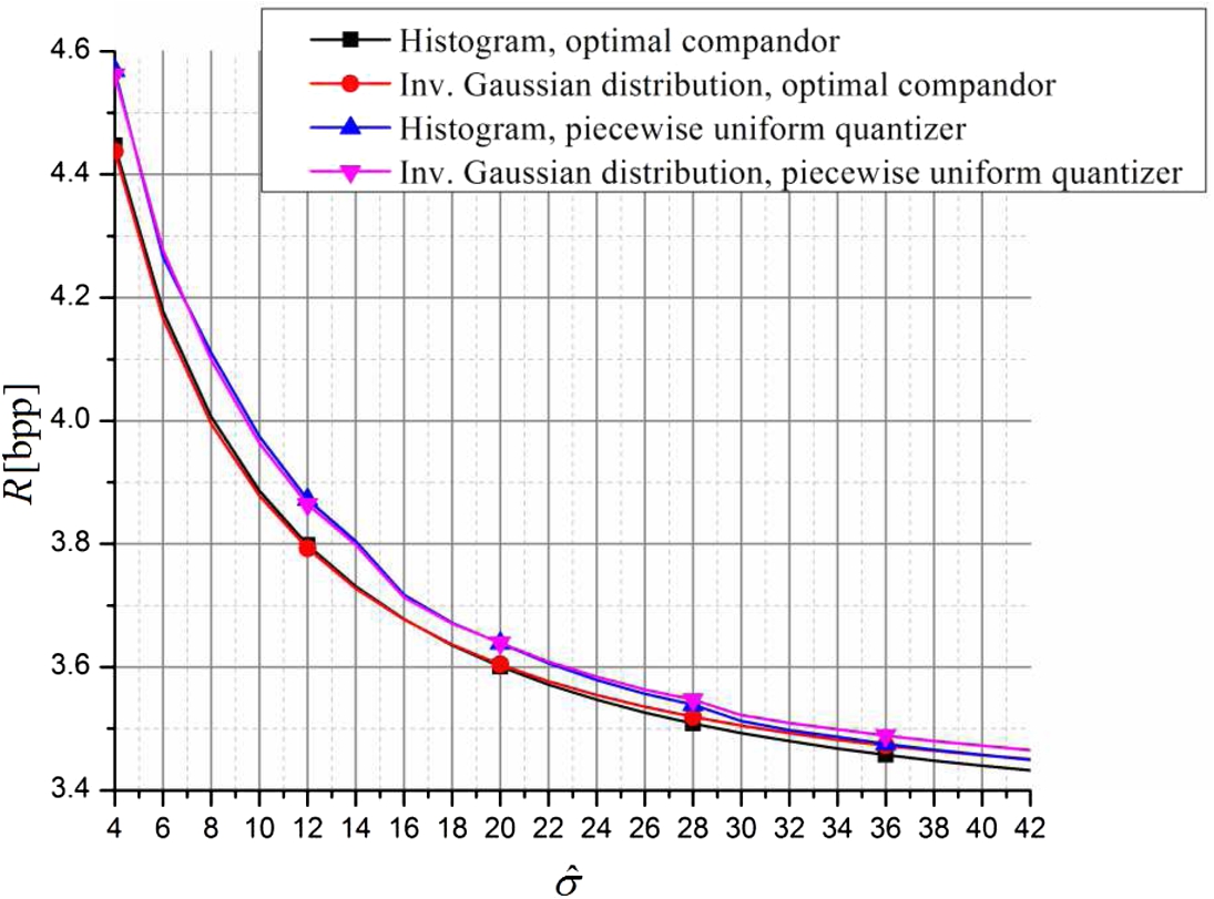
Fig. 5
The total average bit-rate – analytical model.
Table 1
Comparison of experimental and theoretical results – the total average bit-rate and PSQNR.
|
The total average bit-rate [bpp] |
PSQNR [dB] |
|
M1 model |
M2 model |
Experiments |
Theoretical model |
Experiments |
| $\hat{\sigma }$ |
${R^{\mathrm{hist}}}$ |
${R^{\mathrm{Inv}.\hspace{2.5pt}\mathrm{Gaus}}}$ |
${R^{\mathrm{hist}}}$ |
${R^{\mathrm{Inv}.\hspace{2.5pt}\mathrm{Gaus}}}$ |
${R^{\mathrm{ex}}}$ |
${\mathit{PSQNR}^{\mathrm{hist}}}$ |
${\mathit{PSQNR}^{\mathrm{Inv}.\hspace{2.5pt}\mathrm{Gauss}}}$ |
${\mathit{PSQNR}^{\mathrm{ex}}}$ |
| 12 |
3.8720 |
3.8643 |
3.7985 |
3.7924 |
3.9257 |
42.8945 |
43.8275 |
40.1194 |
| 14 |
3.8044 |
3.7986 |
3.7311 |
3.7276 |
3.8987 |
42.9537 |
43.8193 |
40.8063 |
| 15 |
3.7547 |
3.7501 |
3.7031 |
3.7009 |
3.8694 |
41.6060 |
42.3193 |
41.3739 |
| 16 |
3.7171 |
3.7135 |
3.6781 |
3.6772 |
3.8360 |
41.6322 |
42.0689 |
41.0867 |
| 24 |
3.5793 |
3.5842 |
3.5471 |
3.5546 |
3.6572 |
40.0148 |
39.9896 |
40.9050 |
| 30 |
3.5121 |
3.5220 |
3.4931 |
3.5050 |
3.5733 |
38.3763 |
38.2929 |
39.6773 |
In order to compare obtained results with existing models, firstly we provide comparison with the results published in Savic
et al. (
2012). The corresponding theoretical results from the aforementioned paper, for fixed piecewise uniform quantizer application, are
${\mathit{PSQNR}_{\mathrm{inf}}}=35.32$ dB and
${R_{\mathrm{inf}}}=4.375$ bpp. Considering M1 model and taking into account that
PSQNR values increase/decrease for 5.5 dB by changing the bit-rate for 1 bit for medium bit-rates, the proposed system achieves theoretical gain of
PSQNR/R ratio in comparison to the corresponding design presented in Savic
et al. (
2012) and it is shown in Fig.
6.
It can be clearly seen that the proposed modelling provides gain estimation very close to the one obtained by using the exact histogram ($\Delta <1$ dB) for the values of discrete variance $\hat{\sigma }>12$. Moreover, the difference decreases by increasing $\hat{\sigma }$ and the best performance is achieved in the range $\hat{\sigma }\in (14,16)$. It should be noted that for $\hat{\sigma }>22$ difference is lower than 0.25 dB, that is almost negligible.
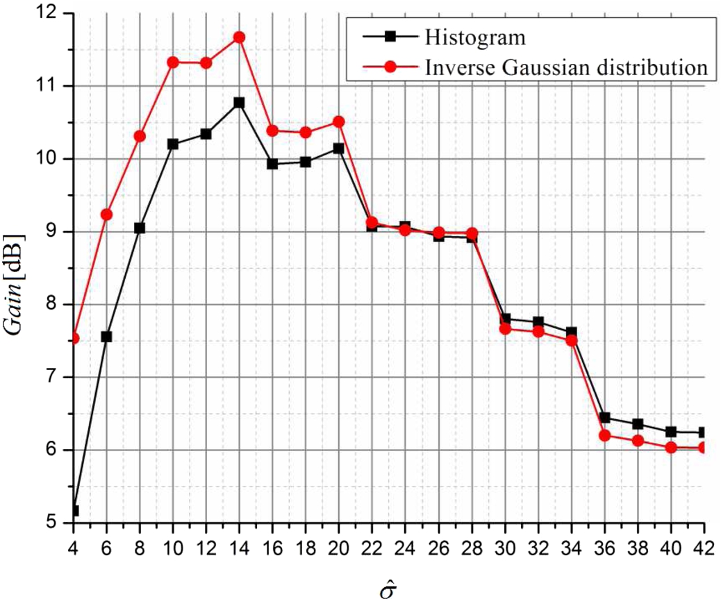
Fig. 6
Theoretical gain – comparison with Savic
et al. (
2012)
$N=16$,
$L=8$.
Consequently, taking into account that the best performance is predicted in the range
$\hat{\sigma }\in (14,16)$ we have decided to provide experimental results by using the proposed algorithm for
$\hat{\sigma }\in (12,14,15,16,24,30)$ and these results and corresponding comparison with the theoretical models are shown in Table
1.
By observing the results shown in Table
1, it can be concluded that the total average bit-rate decreases by increasing discrete designing variance
$\hat{\sigma }$. It is evident that theoretical results obtained by using the proposed solutions (
${R^{\mathrm{Inv}.\hspace{2.5pt}\mathrm{Gaus}}}$) achieve performance very close to the one obtained by using the exact histogram (
${R^{\mathrm{hist}}}$) as well as very close to the experimental results (
${R^{\mathrm{ex}}}$). However, the results obtained by using M1 model are closer to the experimental results as it could be expected because of its higher complexity. Next, the results tell us that for
$\hat{\sigma }\in (15,16,24)$ the absolute errors between the experimental results
$({\mathit{PSQNR}^{\mathit{ex}}})$ and the proposed closed-form solutions
$({\mathit{PSQNR}^{\mathrm{Inv}.\hspace{0.1667em}\mathrm{Gauss}}})$ are less than 1 dB. Furthermore, we can conclude that theoretical results follow the changes of experimental results. This means that the proposed model provides satisfactory performance estimation within the range
$\hat{\sigma }\in (15,30)$. Taking into account results from Fig.
6, it can be concluded that the best system performance is achieved for
$\hat{\sigma }=15$. Moreover, since for
$\hat{\sigma }\in (15,16,24)$ higher accuracy is provided, for all the other numbers of quantization segments
L and quantization levels
N, we will provide analysis that incorporates those three values.
Table
2 shows theoretical and experimental performance for the various values of system parameters.
Table 2
The total average bit-rate and PSQNR for various values of N and L.
| N |
L |
$\hat{\sigma }$ |
${R^{\mathrm{hist}}}$ [bpp] |
${R^{\mathrm{Inv}.\hspace{0.1667em}\mathrm{Gauss}}}$ [bpp] |
${R^{\mathrm{ex}}}$ [bpp] |
${\mathit{PSQNR}^{\mathrm{hist}}}$ [dB] |
${\mathit{PSQNR}^{\mathrm{Inv}.\hspace{0.1667em}\mathrm{Gauss}}}$ [dB] |
${\mathit{PSQNR}^{\mathrm{ex}}}$ [dB] |
| 16 |
4 |
15 |
4.6771 |
4.6838 |
4.4271 |
40.8748 |
41.5134 |
40.8935 |
|
|
24 |
4.5268 |
4.5427 |
4.3802 |
37.6488 |
38.0756 |
39.1120 |
|
|
30 |
4.4748 |
4.4952 |
4.3654 |
36.1054 |
36.4777 |
37.8268 |
| 32 |
4 |
15 |
5.6553 |
5.6720 |
5.4179 |
45.6322 |
46.3163 |
45.4106 |
|
|
24 |
5.5130 |
5.5379 |
5.3710 |
43.3062 |
43.8258 |
44.2079 |
|
|
30 |
5.4549 |
5.4850 |
5.3563 |
42.5318 |
43.0339 |
43.0973 |
|
8 |
15 |
4.7340 |
4.7393 |
4.6939 |
46.6803 |
47.4487 |
46.3190 |
|
|
24 |
4.5525 |
4.5670 |
4.5379 |
45.4434 |
45.9896 |
45.2847 |
|
|
30 |
4.4987 |
4.5177 |
4.4839 |
43.7051 |
44.1817 |
45.3434 |
|
16 |
15 |
4.4131 |
4.3769 |
4.3364 |
46.7983 |
47.5733 |
46.6716 |
|
|
24 |
4.0102 |
3.9907 |
3.9568 |
45.5497 |
46.0716 |
45.8032 |
|
|
30 |
3.8550 |
3.8423 |
3.8180 |
43.8754 |
44.3203 |
45.8192 |
As it was expected, PSQNR value increases by increasing the number of quantization levels. Moreover, for fixed number of quantization levels, PSQNR value increases by increasing the number of segments L. In order to compare compression quality for aforementioned quantizers, the total average bit-rate depending on the number of quantization levels and the number of quantization segments is also shown.
4.1 Comparison of the Obtained Results with Other Models
This section provides comparison of the obtained results with the corresponding one presented in other papers (Savic
et al.,
2012; Mathews and Nair,
2015; Savic
et al.,
2015). The results are compared with the similar techniques as well as with the other that incorporates adaptation and linear prediction. In Table
3 are shown the average
PSQNR and the total average bit-rate values for three standard test grayscale images (Lena, Street and Boat) processed by the proposed algorithm and they are compared with the corresponding results published in Savic
et al. (
2012), denoted with
${\mathit{PSQNR}^{\mathrm{Inf}}}$ and
${R^{\mathrm{Inf}}}$.
In Table
3, with
${\mathit{Gain}^{\mathrm{d}}}$ is denoted experimental gain of the proposed model produced by the proposed quantizer design implementation, whereas
${\mathit{Gain}^{\mathrm{tot}}}$ is the total gain that is obtained by both different quantizer design and variable length Golomb–Rice coding, i.e. achieved by the proposed encoder design. It should be noted that Golomb–Rice coding is not suitable in the case when
$L=4$ since the total average bit-rate is higher than the bit-rate required for fixed quantizers (Savic
et al.,
2012). However, it can be clearly seen that the proposed encoder design provides gain for the all observed system parameters and that the gain reaches 11.56 dB.
Table 3
The comparison of the system performance with the results published in Savic
et al. (
2012) for three standard test grayscale images (Lena, Street and Boat).
| N |
L |
$\hat{\sigma }$ |
${\mathit{PSQNR}^{\mathrm{ex}}}$ [dB] |
${R^{\mathrm{ex}}}$ [bpp] |
${\mathit{PSQNR}^{\mathrm{Inf}}}$ [dB] |
${R^{\mathrm{Inf}}}$ [bpp] |
${\mathit{Gain}^{\mathrm{d}}}$ [dB] |
${\mathit{Gain}^{\mathrm{total}}}$ [dB] |
| 16 |
4 |
15 |
42.045 |
4.504 |
33.037 |
4.375 |
9.008 |
8.299 |
|
|
24 |
39.963 |
4.435 |
|
|
6.926 |
6.596 |
|
|
30 |
38.468 |
4.412 |
|
|
5.431 |
5.228 |
|
8 |
15 |
42.831 |
3.869 |
35.817 |
4.375 |
7.014 |
9.797 |
|
|
24 |
41.895 |
3.657 |
|
|
6.078 |
10.027 |
|
|
30 |
40.443 |
3.573 |
|
|
4.626 |
9.037 |
| 32 |
4 |
15 |
46.556 |
5.496 |
40.058 |
5.375 |
6.498 |
5.833 |
|
|
24 |
45.311 |
5.432 |
|
|
5.253 |
4.940 |
|
|
30 |
44.065 |
5.408 |
|
|
4.007 |
3.826 |
|
8 |
15 |
47.778 |
4.704 |
42.380 |
5.375 |
5.398 |
9.089 |
|
|
24 |
46.177 |
4.490 |
|
|
3.797 |
8.665 |
|
|
30 |
46.225 |
4.490 |
|
|
3.845 |
8.713 |
|
16 |
15 |
48.214 |
4.631 |
42.640 |
5.375 |
5.574 |
9.666 |
|
|
24 |
46.502 |
4.162 |
|
|
3.862 |
10.534 |
|
|
30 |
46.494 |
3.974 |
|
|
3.854 |
11.560 |
Unlike conventionally designed classic block truncation coding models, there are a lot of modifications designed to provide specific performance. In Mathews and Nair (
2015) an adaptive block truncation technique, that uses edge-based quantization in order to improve compression ratio and preserve reconstructed image quality was proposed. The main idea of this kind of adaptation is to adjust quantization levels for block processing depending on whether the observed block contains an edge or not. The authors have designed the system that preserves the edge information, since artifacts near edges are a common phenomenon and edges are considered as a very important feature of an image. From Mathews and Nair (
2015) it can be seen that their model achieves
$\mathit{PSQNR}=36.9919$ dB and compression ratio
$\mathit{CR}=3.1087$ for the standard test grayscale image Lena whereas
$\mathit{PSQNR}=36.3085$ dB and compression ratio
$\mathit{CR}=2.8586$ for the standard test grayscale image Street is achieved. If we calculate the total average bit-rate from those
$\mathit{CR}$ values, we get
$R=2.5734$ bpp for Lena and
$R=2.7986$ bpp for Street. On the other hand, by processing these images with the proposed algorithm for the case
$N=32$,
$L=16$ and
$\hat{\sigma }=30$ (the highest obtained gain) we obtain the following performance – Lena:
$\mathit{PSQNR}=46.624$ dB and
$R=3.721$ bpp; Street:
$\mathit{PSQNR}=46.258$ dB,
$R=3.852$ bpp. By comparing these results with the corresponding one published in Mathews and Nair (
2015), we can conclude that our model achieves higher
$\mathit{PSQNR}$ but also higher average bit-rate. In order to compare the
$\mathit{PSQNR}/R$ ratio, it should be noted that
$\mathit{PSQNR}$ value increases/decreases for 5.5 dB by changing the total average bit-rate for 1 bpp (Savic
et al.,
2012). This way, by transforming the results from Mathews and Nair (
2015) to the same bit-rates as ours, we get corresponding performance: Lena –
$\mathit{PSQNR}=43.3037$ dB,
$R=3.721$ bpp; Street –
$\mathit{PSQNR}=42.1022$ dB,
$R=3.852$ bpp. By comparing these transformed results with the corresponding one from the model that we propose, it can be concluded that the proposed design achieves gain for image Lena
${\mathit{Gain}_{\mathrm{Lena}}}=3.3203$ dB and for image Street
${\mathit{Gain}_{\mathrm{Street}}}=4.1558$ dB.
Next, we provide comparison to the results published in Savic
et al. (
2015), where an application of linear prediction and dual-mode quantization in classic BTC algorithm is presented. The obtained results in Savic
et al. (
2015) for
$N=16$, which is the most suitable configuration since linear prediction provides better performance for lower bit-rates, is
$\mathit{PSQNR}=32.83$ dB and
$R=2.71$ bpp. On the other hand, from Table
3 it can be seen that for
$N=16$,
$L=8$ and
$\hat{\sigma }=15$ we have
$\mathit{PSQNR}=42.831$ dB and
$R=3.8694$ bpp. By transforming the results from Savic
et al. (
2015), taking into account aforementioned
$\mathit{PSQNR}/R$ rule, we have obtained
$\mathit{PSQNR}=39.2067$ dB and
$R=3.8694$ bpp. Finally, we can conclude that the proposed model achieves gain of
${\mathit{Gain}_{\mathrm{eswa}}}=42.83139.2067=3.6243$ dB in comparison to the model that incorporates linear prediction from Savic
et al. (
2015).
In the end, we provide a comparison of the obtained theoretical results obtained for the considered set of ten standard test grayscale images (Tables
1 and
2) with the experimental results for standard test grayscale images that do not belong to the set used for model making. This way we want to show generality of the proposed analytical model and closed-form expressions. Experiments are done for 4 standard test grayscale images – Parrot, Clown, Fruits and Girl. These images are shown in Fig.
7.
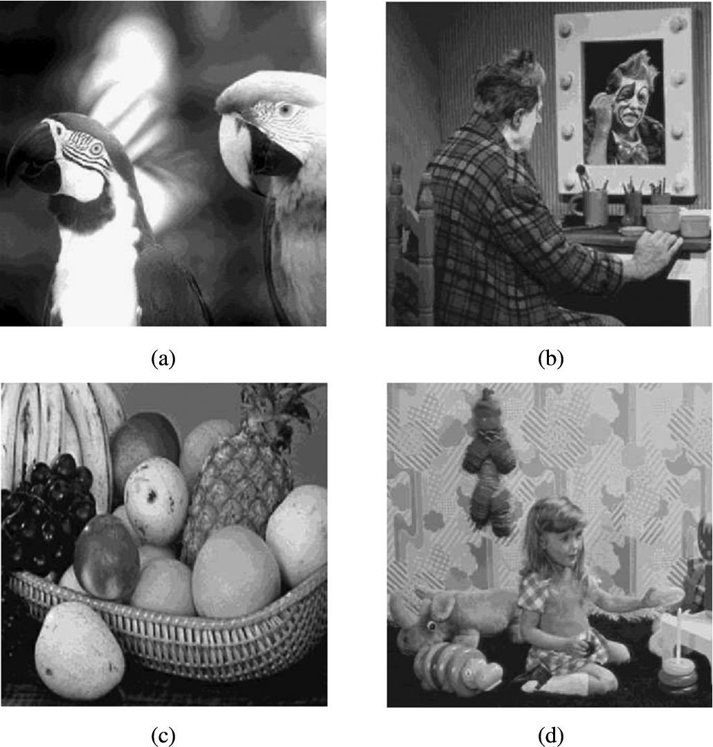
Fig. 7
Standard test grayscale images: (a) Parrot; (b) Clown; (c) Fruits; (d) Girl.
In Table
4 obtained average experimental results (denoted with
${\mathit{PSQNR}^{\mathrm{ex}}}$ and
${R^{\mathrm{ex}}}$) and corresponding theoretical results obtained by using the proposed analytical model (denoted with
${\mathit{PSQNR}^{\mathrm{th}}}$ and
${R^{\mathrm{th}}}$) are shown.
Table 4
System performance for standard test grayscale images from Fig.
7. (
$L=8$;
$\hat{\sigma }=15$).
| N |
${\mathit{PSQNR}^{\mathrm{ex}}}$ |
${R^{\mathrm{ex}}}$ |
${\mathit{PSQNR}^{\mathrm{th}}}$ |
${R^{\mathrm{th}}}$ |
${\Delta _{\mathrm{PSQNR}}}$ [dB] |
${\Delta _{\mathrm{R}}}$ [bpp] |
| 16 |
42.4828 |
3.7235 |
42.3193 |
3.7501 |
0.1635 |
0.0266 |
| 32 |
47.1250 |
4.7145 |
47.4487 |
4.7393 |
0.3237 |
0.0248 |
In Table
4, with
${\Delta _{\mathrm{PSQNR}}}$ and
${\Delta _{\mathrm{R}}}$ are denoted the absolute error rates between corresponding experimental and theoretical results. By observing Table
4, it can be unambiguously seen that the proposed analytical model predicts system performance very well (
${\Delta _{\mathrm{PSQNR}}}\ll 1$ dB,
${\Delta _{\mathrm{R}}}\ll 0.2$ bpp) even for the wider set of standard test grayscale images, whose statistical properties were not taken into consideration and model designing. The reconstructed images obtained by processing with the proposed algorithm are shown in Fig.
8. It can be noticed that the visual difference between reconstructed and original images almost does not exist and that there is not any noticeable geometric irregularity such as block effect.
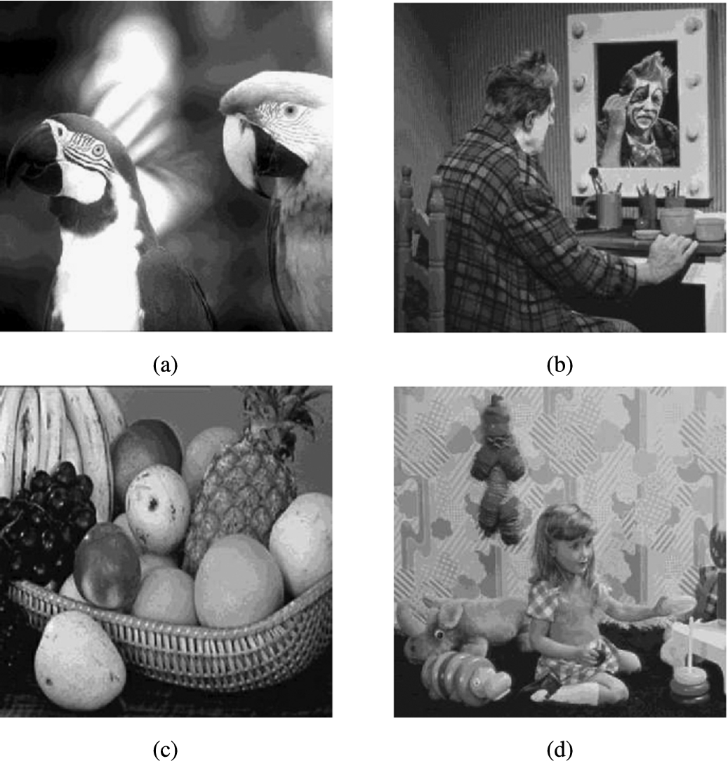
Fig. 8
Reconstructed standard test grayscale images from Fig.
7 (
$N=16$;
$L=8$;
$\hat{\sigma }=15$): (a) Parrot; (b) Clown; (c) Fruits; (d) Girl.
5 Conclusions
BTC algorithm as one of the core techniques for image processing has been modified and upgraded in a number of papers. Also, there are various modifications that are application dependent and they provide satisfactory results in comparison to the other techniques. However, the deficiency of analytical models for performance analysis motivated us to provide a model as well as an improved system design for grayscale image compression. In this study, we have developed the analytical model based on application of Inverse Gaussian distribution. The proposed closed-form solutions for PSQNR and the total average bit-rate provide matching with the experimental results for various values of system parameters within the range of 1 dB and 0.2 bpp, respectively.
Furthermore, the experimental results show that the proposed design provides better performance of reconstructed images in comparison to the other solutions based on the fixed piecewise uniform quantizer. Firstly, comparing with Savic
et al. (
2012), it was shown that experimental gain is provided for various system configurations and it is between 3.826 dB and 11.56 dB. Moreover, the proposed application of Golomb–Rice encoding provides gain even comparing to the other techniques such as adaptation and linear prediction. Comparing the achieved results with the corresponding one from Mathews and Nair (
2015) for two standard test images Lena and Street, we have shown that the proposed system provides gain up to 4.1558 dB. This way, we have concluded that the proposed design achieves better
PSQNR/R ratio in comparison to edge-based adaptation. Also, we have shown that the proposed design provides gain of 3.6243 dB in comparison to the algorithm which apply linear prediction scheme (Savic
et al.,
2015). The proposed method has very low complexity and it provides much lower processing time. In future work, we will intend to research possible application of the proposed quantizer to the other algorithms that incorporate transform coding as well as to provide analytical models for different image processing algorithms due to its deficiency.

