Abstract
Radiologists need to find a position of a slice of one computed tomography (CT) scan in another scan. The image registration is a technique used to transform several images into one coordinate system and to compare them. Such transversal plane images obtained by CT scans are considered, where ribs are visible, but it does not lessen the significance of our work because many important internal organs are located here: liver, heart, stomach, pancreas, lungs, etc. The new method is developed for registration based on the mathematical model describing the rib-bounded contour. Parameters of the mathematical model and of distribution of the bone tissue on the CT scan slice form a set of features describing a particular slice. The registration method applies translation, rotation, and scaling invariances. Several strategies of translation invariance and options of the unification of scales are proposed. The method is examined on real CT scans seeking for its best performance.
1 Introduction
Image analysis becomes a top technology assisting to make decisions in medicine. Images come from various sources: radiology, echoscopy, magnetic resonance, thermovision, tomography, etc. Many diseases may be diagnosed and their treatment observed using the computed tomography (CT) that is a technology allowing the inside of objects to be spatially viewed, using computer-processed X-rays. CT scans are 3D images, i.e. a collection of 2D images (slices), representing human body cross-section with a transversal plane. Such collections of images require special methods and means to handle graphical data, e.g. image segmentation, medical modelling, image registration.
The image registration is a technique used to transform several images into one coordinate system. Although it has applications in many fields, the medical image registration is important among them for aligning and comparing different images (Treigys
et al.,
2008; Oliveira and Tavares,
2012). When evaluating the efficiency of treatment or progress of the disease, pre- and post-treatment, CT scans must be made (for the same patient) and compared by aligning (registering) these two (or more) scans or particular slices from the scans.
In Graf
et al. (
2011), the problem of registering CT scans in a body atlas has been considered. It is also required for navigating automatically to certain regions of a scan or if sub-volumes have to be identified automatically. Various methods are developed for problems of such type (Emrich
et al.,
2010; Feulner
et al.,
2009; Fernández
et al.,
2014). An automated method is developed in Shi
et al. (
2007) in order to identify the corresponding nodules in serial thoracic CT scans for interval change analysis. The method uses rib centrelines as a reference for the initial nodule registration. The rib anatomy is used as a reference point in the CT scan analysis. In Kindig and Kent (
2013), a model is introduced to describe the centroidal path of a rib (i.e. the sequence of centroids connecting adjacent cross-sections) in terms of several physically-meaningful and intuitive geometric parameters in CT scans. This model addresses a critical need for the accurate characterization of rib geometry in the biomechanics literature. A six-parameter shape model of the human rib centroidal path using logarithmic spirals is proposed in Holcombe
et al. (
2016).
When analysing transversal plane images, obtained by computer tomography scans, the peculiarity of the problem is that parts of different ribs are visible on the same slice. It is the reason why the models in Kindig and Kent (
2013) and Holcombe
et al. (
2016) cannot be applied here. The problem arises in selecting a proper function defining a contour, bounded by the fragments of the rib bone in the slice. These fragments are a result of the cross-section of a bone with the transverse plane. The slices may be compared using the bone tissue areas from the cross-section of bones in the slice. The authors in Bilinskas
et al. (
2015) and Bilinskas
et al. (
2017) offer a cardioid-type curve defining the rib-bounded contour on the slice. However, it is not the only one possible. A snake-type curve may serve as an alternative (Kass
et al.,
1988), but computing of such a curve will face problems in the spine area.
This research deals with CT scan slice registration, based on the mathematical model that describes the ribs-bounded contour developed in Bilinskas
et al. (
2017), where a method for analysing transversal plane images, obtained by computer tomography scans, is presented. Such a mathematical model was created and the problem of approximation is solved by finding out the optimal parameters of the model in the least-squares sense. The authors of paper (Bilinskas
et al.,
2017) disclose the problems that appear in building the proper model. Only slices, where ribs are visible, are considered. The methods of analysis of this part of the body are important because many internal organs are located here: liver, heart, stomach, pancreas, lungs, etc. The model is flexible and describes the rib-bounded contour independently of the patient age, sex, and disease.
The registration problem could be solved by using the meta data of the DICOM header of a CT scan. However, the available information is often error-prone. Güld
et al. (
2002) report that several entries in the DICOM header are often imprecise or even completely wrong.
The goal of this paper is to develop a registration method where the model of the rib-bounded contour serves as the basis of the similarity criterion of images (slices). In this case, we have a method of the feature-based registration. The problem is to find the most relevant slice in one scan to the chosen slice from another scan of the same patient. Registration of slices must be done independently of the patient position on the bed and of the radiocontrast agent injection. Feature-based methods find a correspondence between image features, such as points (Bouguet,
2000), or even contours (Li
et al.,
1995). In our case, parameters of the mathematical model and of distribution of the bone tissue on the CT scan slice form a set of features describing a particular slice.
2 The Model
In Bilinskas
et al. (
2017), a method is proposed for bone tissue segmentation and further development of the mathematical model of the tissue configuration in a particular slice. Let us denote a set of bone tissue pixels of the slice by
$B=\{({b_{1i}},{b_{2i}}),\hspace{2.5pt}i=\overline{1,m}\}$. Bilinskas
et al. (
2017) is not the only possibility to extract the bone tissue from the slice, see e.g. Banik
et al. (
2010), Zhang
et al. (
2012). The bone tissue is approximated by a mathematical model. The model consists of two parts. The first part is a modification of cardioid, the second one is a supplement to reduce the spine influence. The first part of the model is described as follows:
Here
s defines the spine cave ‘strength’,
c is the ‘strength’ of subtrahend for breastbone,
l is the steepness of subtrahend for breastbone,
a and
b are horizontal and vertical zoom respectively,
θ is the rotation of the human body, and
$({x_{0}},{y_{0}})$ is the starting point (the ‘spike’ point of the model, see Fig. 1).
The second part of the model is a line-segment bounded by two points
where
${\min _{y}}={\min _{\varphi }}({y_{0}}+b\rho (\varphi )\sin \varphi )$. This part was used seeking a better accuracy of model (1)–(3).
Mathematical model (1)–(4) is defined by an array of 8 parameters
$M=\langle s,c,l,a,b,\theta ,{x_{0}},{y_{0}}\rangle $, the values of which are found by least-squares (Bilinskas
et al.,
2017). The resulting model is shown in Fig.
1.
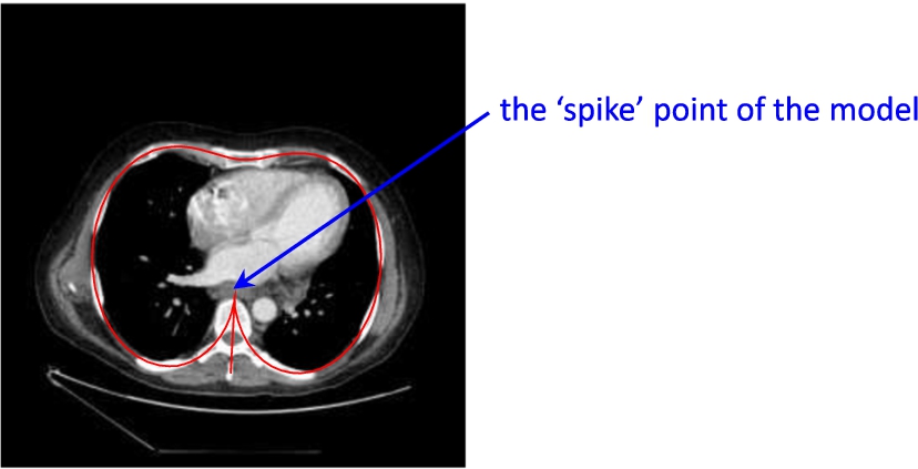
Fig. 1
An example of CT scan slice with a model curve (red line).
3 The Problem of Registration in CT Image Analysis
Radiologists need to find a position of a slice of one CT scan in another scan. Formally, having a slice
${A^{\prime }}$ of scan
${\boldsymbol{A}^{\prime }}$, we should compare it with all the slices in scan
${\boldsymbol{A}^{\prime\prime }}$ and find the most similar slice
${A^{\prime\prime }_{k}}$, i.e. the nearest slice from scan
${\boldsymbol{A}^{\prime\prime }}$ to
${A^{\prime }}$:
Here the function
$\mathit{dist}$ is a similarity measure of two slices. Some possible functions
$\mathit{dist}$ are discussed below.
${A^{\prime }}$ and ${\boldsymbol{A}^{\prime }}$ are called a source or a reference slice and scan, respectively. ${A^{\prime\prime }}$ and ${\boldsymbol{A}^{\prime\prime }}$ are called a target slice and scan, respectively.
4 Data for Slice Registration
For image registration, we need discrete points of the curve of model (
1)–(
3). Denote the sequence of points by
$\boldsymbol{C}$. If
φ runs through the interval
$[-\pi /2;3\pi /2)$ with a step
$2\pi /n$, we get the sequence
$\boldsymbol{C}=({C_{i}}=({x_{i}},{y_{i}}),\hspace{2.5pt}i=\overline{0,n-1})$ of points of the curve (
1)–(
2), where
${x_{i}}$,
${y_{i}}$ are defined by Eq. (
1) and (
2) respectively,
${x_{i}}=x(\frac{2\pi }{n}i)$ and
${y_{i}}=y(\frac{2\pi }{n}i)$. The length of the sequence
$\boldsymbol{C}$ is
n because the second part of the model (a line segment) is not used here.
Some registration methods need weights of model curve points. Weights are gathered by distributing bone tissue points among the curve points $({x_{i}},{y_{i}})$, $i=\overline{0,n-1}$. n groups of bone tissue points are formed. Model points $({x_{i}},{y_{i}})$, $i=\overline{0,n-1}$ have weights $W=({w_{0}},{w_{1}},\dots ,{w_{n-1}})$, where ${w_{i}}$ is the number of bone tissue points in the ith group; the ith group contains points closer to the model point $({x_{i}},{y_{i}})$ than $({x_{j}},{y_{j}})$, $\forall j\ne i$. Without loss of generality, further we will use $W=({w_{0}},{w_{1}},\dots ,{w_{n-1}})$ as normalized weights, where ${\textstyle\sum _{i=0}^{n-1}}{w_{i}}=1$.
Finally, for each slice, we have a set of bone tissue pixels (points)
B, the sequence
$\boldsymbol{C}$ of discrete points of the curve of model (
1)–(
3), array
M of 8 parameters describing the mathematical model, and weights
W of model curve points. Registration is applied to two slices. Denote
B,
$\boldsymbol{C}$,
M, and
W of the source slice by
${B^{\prime }}$,
${\boldsymbol{C}^{\prime }}$,
${M^{\prime }}$, and
${W^{\prime }}$, and that of target slice by
${B^{\prime\prime }}$,
${\boldsymbol{C}^{\prime\prime }}$,
${M^{\prime\prime }}$, and
${W^{\prime\prime }}$, e.g.
${W^{\prime }}=({w^{\prime }_{0}},{w^{\prime }_{1}},\dots ,{w^{\prime }_{n-1}})$ are the weights of the source slice model, and
${W^{\prime\prime }}=({w^{\prime\prime }_{0}},{w^{\prime\prime }_{1}},\dots ,{w^{\prime\prime }_{n-1}})$ are the weights of the target slice model.
5 Registration
The registration method below applies translation, rotation, and scaling invariance. These invariances are usual in the image registration (Szeliski,
2006). However, their realization depends on a particular target area.
The comparison of slices is based on:
5.1 Rotation Invariance
Model (
1)–(
3) has a parameter
θ, describing the rotation of a patient with respect to the bed. This parameter indicates the rotation of the model curve about the point
$({x_{0}},{y_{0}})$ as well. Rotation invariance is realized rotating the model curve about the point
$({x_{0}},{y_{0}})$ by the angle
$-\theta $. This procedure should be applied both to source and target slices. The revised parameters of the models become
${M^{\prime }}=\langle {s^{\prime }},{c^{\prime }},{l^{\prime }},{a^{\prime }},{b^{\prime }},0,{x^{\prime }_{0}},{y^{\prime }_{0}}\rangle $ and
${M^{\prime\prime }}=\langle {s^{\prime\prime }},{c^{\prime\prime }},{l^{\prime\prime }},{a^{\prime\prime }},{b^{\prime\prime }},0,{x^{\prime\prime }_{0}},{y^{\prime\prime }_{0}}\rangle $. Without loss of generality and seeking for simplicity of notation, we redefine
$\boldsymbol{C}$ by the sequence of points after the rotation described above, where entire points from
$\boldsymbol{C}$ are rotated by
$-\theta $ about
$({x_{0}},{y_{0}})$. Therefore, in the further text, the sequences after rotations of source and target slices are denoted as
${\boldsymbol{C}^{\prime }}=(({x^{\prime }_{i}},{y^{\prime }_{i}}),\hspace{2.5pt}i=\overline{0,n-1})$ and
${\boldsymbol{C}^{\prime\prime }}=(({x^{\prime\prime }_{i}},{y^{\prime\prime }_{i}}),\hspace{2.5pt}i=\overline{0,n-1})$, respectively.
5.2 Scale Invariance
Most often the compared CT scan slices have a different scale. The scale depends on the parameters of CT scanner. These parameters may vary in different scans. One of such parameters is the size of a pixel of the image.
In our model, we have scale parameters
a and
b (see Eqs. (
1) and (
2)). For comparison of two slices, the parameters
a and
b of these slices should be scaled. Large scale invariance may be attained varying
a and
b. Therefore, the pyramid technique (Burt,
1981) has no use here. Three options O1, O2, and O3 of the unification of scales are considered below. Options O2 and O3 are used when DICOM metadata tags are not precise or are even lost.
The first option O1 is the usage of DICOM metadata tags, indicating the size of pixel. Let a pixel be quadratic. Denote the width of the source slice pixel by ${z^{\prime }}$, and that of the target slice pixel by ${z^{\prime\prime }}$. The revised parameters of the source slice model are ${M^{\prime }}=\langle {s^{\prime }},{c^{\prime }},{l^{\prime }},{a^{\prime }}\cdot {z^{\prime }}/{z^{\prime\prime }},{b^{\prime }}\cdot {z^{\prime }}/{z^{\prime\prime }},0,{x^{\prime }_{0}},{y^{\prime }_{0}}\rangle $. The parameters of target slice remain unchanged: ${M^{\prime\prime }}=\langle {s^{\prime\prime }},{c^{\prime\prime }},{l^{\prime\prime }},{a^{\prime\prime }},{b^{\prime\prime }},0,{x^{\prime\prime }_{0}},{y^{\prime\prime }_{0}}\rangle $.
The next two options take into account the specificity of the problem, the source and target slices are of the same patient. In these cases, the scaling is performed using specific features of the curve describing the bone tissue:
O2) the maximal width of the region, bounded by the curve,
O3) the area of the region, bounded by the curve.
If the maximal width is considered (O2), then the target slice model remains as it stands, and the parameters of the source slice model are revised as follows:
If the area of the region bounded by the curve is considered (O3), then the target slice model remains as it stands, and the parameters of the source slice model are revised as follows:
The efficiency of registration is examined experimentally in this paper, using different options O1, O2 and O3.
Without loss of generality and seeking for simplicity of notation, we redefine $\boldsymbol{C}$ by the sequence of points after scaling described above. Therefore, in the further text, the sequences after scaling the source and target slices are denoted as ${\boldsymbol{C}^{\prime }}=(({x^{\prime }_{i}},{y^{\prime }_{i}}),i=\overline{0,n-1})$ and ${\boldsymbol{C}^{\prime\prime }}=(({x^{\prime\prime }_{i}},{y^{\prime\prime }_{i}}),i=\overline{0,n-1})$, respectively.
5.3 Translation Invariance
There are several reasons generating the necessity to solve the problem of translation invariance. The patient lies in various positions on the bed during different scans, and models, corresponding to target and source slices, differ as usual.
The translation invariance can be realized in two steps: horizontal translation and the following vertical translation.
The models of bone tissue of the source and target slices have a vertical symmetry: the axis of symmetry crosses the abscissa axis at
${x^{\prime }_{0}}$ and
${x^{\prime\prime }_{0}}$ for the source and target slices, respectively. The horizontal translation invariance will be ensured by moving the source slice model as follows:
Note that ${x^{\prime\prime }_{0}}-{x^{\prime }_{0}}=\frac{1}{n}{\textstyle\sum _{i=0}^{n-1}}({x^{\prime\prime }_{i}}-{x^{\prime }_{i}})$, i.e. $\Delta x$ is the average of differences of abscissas of the corresponding source and target points of the model curve. The model, corresponding to the source slice, becomes ${M^{\prime }}=\langle {s^{\prime }},{c^{\prime }},{l^{\prime }},{a^{\prime }}\cdot z,{b^{\prime }}\cdot z,0,{x^{\prime }_{0}}+\Delta x,{y^{\prime }_{0}}\rangle $ that is equivalent to ${M^{\prime }}=\langle {s^{\prime }},{c^{\prime }},{l^{\prime }},{a^{\prime }}\cdot z,{b^{\prime }}\cdot z,0,{x^{\prime\prime }_{0}},{y^{\prime }_{0}}\rangle $.
The problem is more complicated to find optimal $\Delta y$ to move the source slice model vertically. The model curve is not symmetric to any horizontal line and the ‘spike’ of the model may have a different length (${y_{0}}-{\min _{i}}{y_{i}}$) as $\theta =0$: even similar slices can have a large difference of ${y_{0}}$, as the parameter s may slightly compensate it.
Several strategies for finding $\Delta y$ are developed and examined below.
5.3.1 Pointwise Comparison (PW)
The simplest criterion in search of
$\Delta y$ is such that the distances between the
ith source slice model point and the
ith target slice model point were as minimal as possible. The problem may be formulated as a least-squares one:
Derivative of
ϕ is
and solving
$\frac{d\phi }{d\Delta y}=0$ yields
i.e.
$\Delta y$ is the average of differences of ordinates of the corresponding source and target points of the model curve.
The method was tested using two CT scans and searching for optimal positions of slices from the source scan with respect to target scan slices, i.e. applying Eq. (
5) to all slices
${A^{\prime }}$ in scan
${\boldsymbol{A}^{\prime }}$, where
is the sum of squared distances between the corresponding source and target points of model curve in Eq. (
5). Here,
$\Delta x$ is given in Eq. (
8), and
$\Delta y$ is given in Eq. (
11).
A pointwise comparison has disadvantages. Figure
2 shows the example of the source slice model (red line) and the most appropriate target slice model (blue line), indicated by a radiologist. We notice their insufficient matching. It is because the distances between the corresponding source and target model curve points are used in Eq. (
12). By moving the blue curve upwards, we get much better matching (see Fig.
3), but the distance between two corresponding points in different models may grow (two such points are connected with grey line in Figs.
2 and
3). This example indicates that the pointwise comparison is insufficient to find proper
$\Delta y$.
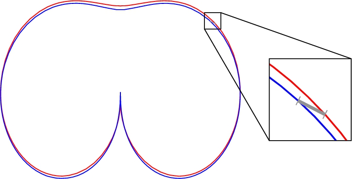
Fig. 2
Red is the source slice model, blue is the correct target slice model, shifted using (
11), and grey is a line between two corresponding points in different models.
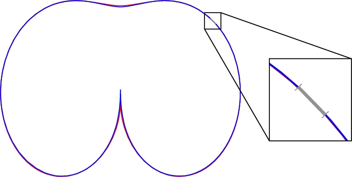
Fig. 3
The same models as in Fig.
2, but with the blue curve shifted slightly above.
5.3.2 Total Least Squares (TLS)
Figure
3 clearly shows that the
ith point of the source slice model should be compared not with the
ith point of the target slice model, but with the nearest point on this model. Therefore, the problem to search for optimal
$\Delta y$ may be formulated as follows:
where
${\overline{y}^{\prime }}({x^{\prime\prime }_{i}},{y^{\prime\prime }_{i}},\Delta x,\Delta y)$ is a function giving the ordinate of the nearest point on the source model curve (shifted by
$(\Delta x,\Delta y)$) from
$({x^{\prime\prime }_{i}},{y^{\prime\prime }_{i}})$. As noted above,
$\Delta x={x^{\prime\prime }_{0}}-{x^{\prime }_{0}}$ ensures the horizontal translation invariance. Therefore, it is applied in Eq. (
13). In the experiments, the source model curve was linearly interpolated between the
n sampled points and problem (
13) was solved using one-dimensional search.
Let the comparison criterion in Eq. (
5) of two slices be as follows:
where
${\overline{x}^{\prime }}({x^{\prime\prime }_{i}},{y^{\prime\prime }_{i}},\Delta x,\Delta y)$ is a function the value of which is an abscissa of the nearest point on the source model curve (shifted by
$(\Delta x,\Delta y)$) from
$({x^{\prime\prime }_{i}},{y^{\prime\prime }_{i}})$.
Some matching examples imply that the result could be improved even more. For example, the models of the source (Fig.
4a) and target (Fig.
4b) slices, where the breastbone is not visible, are expressed in red and blue in Fig.
4c, respectively. The difference between models is in the top middle part of a model, where there is no bone tissue. These models are very similar, where the bone tissue is present. Therefore, a disadvantage of the total least-squares strategy is that it considers, with the same importance, the places of the model, where there is no bone tissue in the slice.
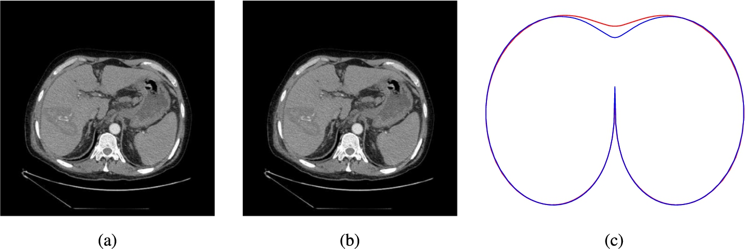
Fig. 4
Source (a) and target (b) slices of the same position, respectively; models of these slices (c).
5.3.3 Weighted Total Least Squares (WTLS)
To solve the problem of the breastbone cave uncertainty, the model curve points, that do not have the bone tissue nearby, must be not included in the comparison of slices. It is done by introducing model point weights, as explained in Section
4. The problem for
$\Delta y$ evaluation becomes as follows:
where
${\overline{w}^{\prime }}({x^{\prime\prime }_{i}},{y^{\prime\prime }_{i}},\Delta x,\Delta y)$ is a function the value of which is the weight of the nearest point on the source model curve (shifted by
$(\Delta x,\Delta y)$) from
$({x^{\prime\prime }_{i}},{y^{\prime\prime }_{i}})$.
$\Delta x={x^{\prime\prime }_{0}}-{x^{\prime }_{0}}$ as above.
${w^{\prime\prime }_{i}}$ is the weight of the point
$({x^{\prime\prime }_{i}},{y^{\prime\prime }_{i}})$ with respect to the density of the bone tissue spread near to this point. In the experiments, the weights
${\overline{w}^{\prime }}({x^{\prime\prime }_{i}},{y^{\prime\prime }_{i}},\Delta x,\Delta y)$ for the source model are linearly interpolated between the sampled points, and problem (
15) was solved using one-dimensional search.
The comparison criterion of two slices is as follows:
The one dimensional search for finding $\Delta y$ may be pointed out as the main disadvantage of the weighted total least squares strategy.
5.3.4 Weighted Ordinary Least Squares (WOLS)
In this strategy, the problem for
$\Delta y$ evaluation is as follows:
Here $\overline{\overline{y}}{\hspace{0.1667em}^{\prime }}({x^{\prime\prime }_{i}},\Delta x)$ is the function the value of which is the ordinate of the source model curve (shifted by $\Delta x$) at the abscissa point ${x^{\prime\prime }_{i}}$, dependently whether the ith point $({x^{\prime\prime }_{i}},{y^{\prime\prime }_{i}})$ of the target model is on top or bottom of the model curve. $\Delta x={x^{\prime\prime }_{0}}-{x^{\prime }_{0}}$ as above. ${w^{\prime\prime }_{i}}$ is the weight of the point $({x^{\prime\prime }_{i}},{y^{\prime\prime }_{i}})$ with respect to the density of the bone tissue spread near to this point. ${\overline{\overline{w}}^{\prime }}({x^{\prime\prime }_{i}},\Delta x)$ is the weight of the point of the source model curve (shifted by $\Delta x$) at the abscissa point ${x^{\prime\prime }_{i}}$, dependently whether the ith point $({x^{\prime\prime }_{i}},{y^{\prime\prime }_{i}})$ of the target model is on top or bottom of the model curve.
In the experiments, the values of functions
$\overline{\overline{y}}{\hspace{0.1667em}^{\prime }}({x^{\prime\prime }_{i}},\Delta x)$ and
$\overline{\overline{w}}{\hspace{0.1667em}^{\prime }}({x^{\prime\prime }_{i}},\Delta x)$ were obtained via a linear interpolation of the known values from the source model. Top and bottom parts were extracted for functions
$\overline{\overline{y}}{\hspace{0.1667em}^{\prime }}$ and
$\overline{\overline{w}}{\hspace{0.1667em}^{\prime }}$ as follows. When
i runs from 0 to
$n-1$, the points
$({x_{i}},{y_{i}})$ lie on the top of the slice model curve starting from such smallest
i (denote it by
${i^{\ast }}$), where
${x_{i+1}}<{x_{i}}$, and ending with such
i (denote it by
${i^{\ast \ast }}$), where
${x_{i+1}}>{x_{i}}$. The bottom curve consists of all the remaining points and has two points
$({x_{{i^{\ast }}}},{y_{{i^{\ast }}}})$ and
$({x_{{i^{\ast \ast }}}},{y_{{i^{\ast \ast }}}})$ common to the top curve. The criterion whether the point
$({x_{i}},{y_{i}})$ lies on the bottom or top of the slice model is illustrated in Fig.
5.
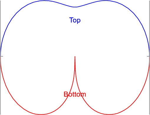
Fig. 5
Division of the model curve into top (blue line) and bottom (red line) parts.
Equation (
17) can be solved analytically, yielding equation (
18):
The comparison criterion of two slices is as follows:
Note that in Eq. (
19) only the weights of model curve points are used.
6 Experiments
Scans of the same patient are examined, where the relative position of one scan is known with respect to the other one. Two pairs of scans with different slice thickness have been examined. The first source scan has 96 slices, the target scan has 106 slices, and slice thickness is 1.25 mm. The second source scan has 53 slices, the target scan has 49 slices, and slice thickness is 2.5 mm. During experiments with the first pair of scans, for each source slice, the most similar slice was found out in the target scan. The correct slice in the target scan is known in advance. Therefore, the registration error may be set to be the absolute difference in millimetres (mm) between the positions on the human body longitudinal axis of two target slices, determined by Eq. (
5) and the correct one.
Table 1
Results of the pointwise comparison (PW) with different scale invariance options.
|
${\varepsilon _{\mathit{mean}}}$ |
σ |
${\varepsilon _{\max }}$ |
| O1 |
6.575 |
8.405 |
36.25 |
| O2 |
9.102 |
11.627 |
47.50 |
| O3 |
9.648 |
11.976 |
47.50 |
Table 2
Results of the total least-squares (TLS) with different scale invariance options.
|
${\varepsilon _{\mathit{mean}}}$ |
σ |
${\varepsilon _{\max }}$ |
| O1 |
9.974 |
9.226 |
38.75 |
| O2 |
10.052 |
14.607 |
60.00 |
| O3 |
8.737 |
13.507 |
60.00 |
While examining our new registration method, for each source slice, the registration error has been evaluated applying four different strategies PW, TLS, WTLS and WOLS of translation invariance and three options O1, O2, and O3 of the unification of scales (see Sections
5.2 and
5.3). The results were averaged through all the source slices. They are the mean error
${\varepsilon _{\mathit{mean}}}$, the error standard deviation
σ, and the maximum error
${\varepsilon _{\max }}$. The results are presented in Tables
1–
4 for various strategies of translation invariance of the first pair of CT scans. The results of weighted ordinary least-squares with invariance option O3 on the second pair of CT scans with 2.5 mm slice thickness are presented in Table
5.
In addition, the experiments were carried out using Pyramidal Implementation of the Lucas Kanade Feature Tracker (Bouguet,
2000) to find features and match them and the RANSAC method (Fischler and Bolles,
1981) in order to find the transformation matrix. It is realized by the
estimateRigidTransform function of OpenCV library. This function is applied to two slices (grayscale images) and the estimated transformation matrix is applied to a set of bone tissue pixels of the target slice (denote the result by
${B^{\ast }}$). Finally, two sets of bone tissue pixels
${B^{\prime }}$ and
${B^{\ast }}$ are compared,
$\mathit{dist}({B^{\prime }};{B^{\ast }})=(|{B^{\prime }}|-|I|+|{B^{\ast }}|-|I|)/(|{B^{\prime }}|+|{B^{\ast }}|)$, where
I is the intersection of
${B^{\prime }}$ and
${B^{\ast }}$,
$|\hspace{0.1667em}\cdot \hspace{0.1667em}|$ is the cardinality of the set. Here the intersection is assumed as the pixel-wise logical AND operator of two binary images
${B^{\prime }}$ and
${B^{\ast }}$. The function
$\mathit{dist}({B^{\prime }};{B^{\ast }})$ returns values from interval
$[0;1]$. The experiments have shown that the examined combination of Pyramidal Implementation of the Lucas Kanade Feature Tracker and RANSAC method is not very accurate, it leads to very poor registration results, as shown in Table
6.
Table 3
Results of the weighted total least-squares (WTLS) with different scale invariance options.
|
${\varepsilon _{\mathit{mean}}}$ |
σ |
${\varepsilon _{\max }}$ |
| O1 |
0.977 |
0.604 |
2.50 |
| O2 |
0.469 |
0.657 |
2.50 |
| O3 |
0.703 |
0.740 |
3.75 |
Table 4
Results of the weighted ordinary least-squares (WOLS) with different scale invariance options.
|
${\varepsilon _{\mathit{mean}}}$ |
σ |
${\varepsilon _{\max }}$ |
| O1 |
0.508 |
0.614 |
1.25 |
| O2 |
0.326 |
0.549 |
1.25 |
| O3 |
0.339 |
0.555 |
1.25 |
Table 5
Results of the weighted ordinary least-squares (WOLS) with invariance option O3 of a pair of CT scans with 2.5 mm slice thickness.
|
${\varepsilon _{\mathit{mean}}}$ |
σ |
${\varepsilon _{\max }}$ |
| O3 |
0.102 |
0.245 |
2.5 |
Table 6
Results of the estimateRigidTransform.
| ${\varepsilon _{\mathit{mean}}}$ |
σ |
${\varepsilon _{\max }}$ |
| 28.53 |
15.54 |
48.75 |
7 Overview of the Results and Conclusions
This research is devoted to the analysis of transversal plane images, obtained by computer tomography scans. A method of the feature-based registration has been developed, where the model of the rib-bounded contour serves as the basis of the similarity criterion of images (slices). The model is flexible and describes the rib-bounded contour independently of the patient age, sex, and disease. We consider the slices where ribs are visible because many important internal organs are located here. The registration method applies translation, rotation, and scaling invariances. Several strategies of translation invariance and options of the unification of image scales are proposed. The method is examined on real CT scans seeking for its best performance. It works well independently of the radiocontrast injection.
The experiments have proved the efficiency of the new registration method, where the configuration of bone tissue is taken into account in the form of a mathematical model.
${\varepsilon _{mean}}$ values in Tables
5 and
6 indicate that such an approach is much more accurate as compared with a combination of Pyramidal Implementation of the Lucas Kanade Feature Tracker and RANSAC method.
${\varepsilon _{\mathit{mean}}}=0.5$ mm is an acceptable error.
The results in Tables
1–
4 indicate that the pointwise comparison and total least-squares strategies fall behind to the weighted total least-squares and weighted ordinary least-squares strategies. These two last strategies have a common peculiarity: they use weights of model curve points, where the weights are evaluated in dependence of the distribution of bone tissue points on the slice. The best strategy uses the weighted ordinary least-squares. The results of the weighted ordinary least-squares strategy are very good both for 1.25 and 2.5 mm slice thickness. Note that this strategy is little dependent on the scale invariance options. This fact leads to the final conclusion that the weights of model curve points play the key role in the efficient registration of thorax CT scan slices.

