Abstract
Medical X-ray images are prevalent and are the least expensive diagnostic imaging method available widely. The handling of film processing and digitization introduces noise in X-ray images and suppressing such noise is an important step in medical image analysis. In this work, we use an adaptive total variation regularization method for removing quantum noise from X-ray images. By utilizing an edge indicator measure along with the well-known edge preserving total variation regularization, we obtain noise removal without losing salient features. Experimental results on different X-ray images indicate the promise of our approach. Synthetic examples are given to compare the performance of our scheme with traditional total variation and anisotropic diffusion methods from the literature. Overall, our proposed approach obtains better results in terms of visual appearance as well as with respect to different error metrics and structural similarity.
1 Introduction
Medical image denoising is an important area within computer aided diagnosis (CAD) systems. One of the well known and very accessible methods for imaging is the X-ray which is used throughout the world. X-ray image is formed when an area under consideration of a patient is exposed under X-rays and resulting attenuation is captured. Now digitization is an important improvement in medical imaging systems and the quantum noise characteristics of the X-ray scattering needs to be taken into account.
Image restoration under different noise types has been widely researched over the past few years and variational and partial differential equation (PDE) based methods are very popular in this regard. One of the widely used methods is that of Rudin
et al. (
1992) which utilizes the total variation (TV) regularization or minimization of the
${L^{2}}$ norm of the gradient image. This TV regularization enjoys nice mathematical properties and prefers piecewise constant solutions. This in turn can be detrimental in medical image denoising as flat (homogenous) regions can be attenuated into piecewise constant regions, an effect known as
staircasing artifacts (Le
et al.,
2007). This is not desirable since noise removal is only a pre-processing step for further image analysis and decision making systems. Therefore, creating artificial regions in medical images is not preferred and better alternatives are sought. One of the important improvement is to use an edge indicator function with TV regularization for stopping staircasing artifacts as well as to inhibit smoothing across edges (Strong and Chan (
1996); Prasath and Singh (
2010),
2012).
Medical X-ray images suffer from quantum noise and we utilize an adaptive TV regularization along with an appropriate image fidelity term for restoring such corrupted images. The quantum noise encountered in X-ray is due to the photons hitting the detector and the finite number of random events are counted, thereby leading to inherent presence in the acquired images. We use the Poisson distribution to model the quantum noise in X-ray imagery and in this paper we study an application of adaptive TV regularization with alternating direction method of multipliers (ADMM) employed for the optimization (Boyd
et al.,
2011; Figueiredo and Biouscas-Dias,
2010). For the adaptive weight we use the generalized inverse gradient term which controls the spread of salient edges with local statistics. By combining this localized edge indicator function via local histograms and inverse gradients with TV regularization, we obtain better regularized images with efficient Poisson noise removal and edge preservation. Experimental results on synthetic and real data indicate our method obtains better results than related regularization models (Le
et al.,
2007; Zhou and Lia,
2012) in terms of image quality metrics and structure preservation.
We organized the paper as follows. Section
2 introduces the proposed adaptive total variation for quantum noise removal. Section
3 provides experimental and comparison results and Section
4 concludes the paper.
2 Adaptive Total Variation Regularization
2.1 Total Variation Regularization
Total variation (TV) regularization is one of the well-known approach in solving the ill-posed inverse problem of image restoration. The main advantage of the TV is that it preserves edges without compromising the quality of denoising capabilities. The TV regularization is written as minimization of the following,
where
$u:\Omega \subset {\mathbb{R}^{2}}\to \mathbb{R}$, and the minimization is taken over a suitable space such as the space of functions of bounded variation
$BV(\Omega )$. Although the TV regularization removes noise while preserving salient edges, it can create artificial edges in homogeneous areas which is terms as ’staircasing’ artifacts. This is an undesirable quality while denoising medical imagery as creating new structures can cause confusions in the final medical diagnostic systems. To avoid the staircasing artifacts while maintaining the important edge preserving property of TV has motivated many studies to come up with adaptive solutions (Prasath
et al.,
2015).
2.2 Proposed Approach
2.2.1 Adaptive total variation
In this paper we assumed that a given grayscale image
${u_{0}}:\Omega \subset {\mathbb{R}^{2}}\to \mathbb{R}$ be corrupted by Poisson noise. We assume the forward model consist of the noisy image
${u_{0}}(x)$:
where
$\Omega \subset {\mathbb{R}^{2}}$ is the image domain (rectangle), and
$x=({x_{1}},{x_{2}})$ pixels, and
u is the latent image, with Poisson distribution for the observed image
$p({u_{0}}|u)={e^{-u(x)}}u{(x)^{{u_{0}}(x)}}/{u_{0}}(x)!$. By combining Poisson noise fidelity term, the general regularization model is written in unconstrained form as Le
et al. (
2007),
In this work, we utilize the adaptive total variation (ATV) regularization with the inverse gradient based edge indicator functions,
where spatially adaptive weight is chosen typically as Strong and Chan (
1996), Prasath and Singh (
2012), Zhou and Lia (
2012),
with
$k>0$ a contrast parameter. However, this inherits some of the drawbacks with other gradient regularizations such as detecting blocky edges, see Fig.
1(b). To improve the performance of the TV regularization and to avoid blocky artifacts, here we propose the following generalized inverse gradient term which incorporates local statistics with patches extracted from the image.
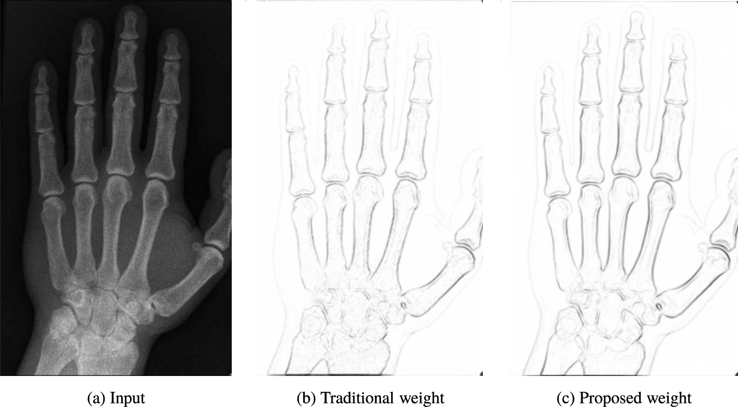
Fig. 1
Using an edge indicator based weights our adaptive TV regularization obtains better noise removal without smoothing out edges. (a) Input image with Poisson noise level unknown. (b) Weights computed using the inverse gradient of the input image, see Eq. (
5), and (c) the proposed generalized inverse gradient of the input image, see Eq. (
9), with parameters
$k=0.06$,
$r=5$,
$\sigma =1$. Both the weights were rescaled to
$[0,1]$ for better visualization.
2.2.2 Generalized inverse gradient weights
Let
${\mathcal{N}_{x,r}}$ be the local region centered at
x with radius
r. Consider the local histogram of a pixel
$x\in \Omega $ and its corresponding cumulative distribution function (Prasath and Delhibabu,
2014),
for
$0\leqslant y\leqslant L$, respectively. Here
$|A|$ denotes the number of elements in the set
A. We define the following local histogram quantity,
which allows us to quantify local regions
${\mathcal{N}_{x,r}}$ of a given image
$u(x)$. The adaptive weight we consider here is then given as,
We used
$r=5$ for the neighbourhood size,
$L=255$ for 8-bit images,
$\sigma =2$ in the Gaussian kernel smoothing in our experiments. The use of local histograms based quantity within the inverse gradient weight improves the edge map with inhibiting the blocky edges and providing a clear discontinuities present in the input image, see Fig.
1(c). The wellposedness of the above adaptive weighted TV regularization based model can be obtained using the theory of calculus of variations (Prasath and Singh,
2012; Prasath
et al.,
2015).
2.3 Alternating Direction Method of Multipliers (ADMM)
To solve the energy minimization problem with weighted TV regularization (
3) we utilize the alternating direction method of multipliers (ADMM) algorithm which is very efficient in terms of computational time. We provide a brief treatment as for the adaptive TV regularization the general ADMM formulation carries over with only little modifications, and we refer to Figueiredo and Biouscas-Dias (
2010) for more details. The following iterative formulations constitute the ADMM for our problem,
Here
λ is the Lagrangian multiplier,
b auxiliary variable, and
$\alpha >0$ is a parameter (with a relation
${\lambda ^{k}}=-\alpha {b^{k}}$). To solve the first minimization problem (weighted TV regularization with
${L_{2}}$ fidelity) for
u various optimization methods can be utilized. In this work, we use Chambolle’s dual minimization method (Chambolle,
2004),
where
p is the dual variable and can be obtained by the following formula,
To solve for
v, a simple solution exists,
3 Experimental Results
3.1 Setup, Parameters, and Error Metrics
We rescaled the images used here to the continuous domain
$[0,1]$. The initial parameters of ADMM and dual minimization
$\alpha =1$,
${b^{t=0}}=0$,
${p^{t=0}}=0$,
$v={u_{0}}$, inner iteration of 5 (for dual variable
p in Eq. (
14)) were set in all our experimental results reported here. For the weights we utilize the pre-smoothing Gaussian kernel with
$\sigma =1$, and the neighbourhood size
$r=5$ (for the local histogram in the proposed generalized inverse gradient weight (
9) in our comparison results. The Lagrangian multiplier
λ and the contrast parameter
k were modified according to optimal results presented below. Typically 20–30 iterations of the ADMM is sufficient to obtain good restoration results on a MATLAB implementation (on a Mac Pro Laptop, 2.3 GHz Intel Core
$i7$ processor, 8 GB 1600 MHz DDR3 memory), and we show the optimized results in the experiments reported below.
For comparing the quality of image restorations in this paper we utilize the root mean squared error (RMSE), relative error (RE), Pratt’s figure of merit (FOM), and structural similarity (SSIM) (Wang
et al.,
2004). These are given as,
where
${u_{\mathrm{o}}}$ is the original (noise-free) image, and the image is of size
$m\times n$.
Pratt’s FOM is calculated as,
where
${E_{\mathrm{a}}}$,
${E_{\mathrm{d}}}$ are the number of actual and detected edge pixels (using the classical Sobel edge detector),
$\gamma =0.1$ scaling parameter fixed. The higher value of FOM indicate better quality edge map and value closer to 1 shows the denoising method has good edge preserving property. The SSIM is calculated between two windows
${\omega _{1}}$ and
${\omega _{2}}$ of common size
$N\times N$, and is given by,
where
${\mu _{{\omega _{i}}}}$ the average of
${\omega _{i}}$,
${\sigma _{{\omega _{i}}}^{2}}$ the variance of
${\omega _{i}}$,
${\sigma _{{\omega _{1}}{\omega _{2}}}}$ the covariance, and
${c_{1}},{c_{2}}$ stabilization parameters. The mean value of SSIM (MSSIM) is taken as the final error metric and if the value is closer to 1 indicating better structural similarity with
${u_{\mathrm{o}}}$ the original image.
3.2 Synthetic Examples
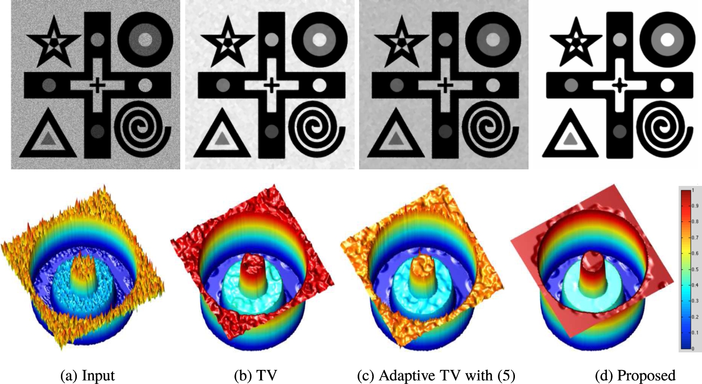
Fig. 2
Comparison of different denoising TV regularization on noisy synthetic
$Shapes$ image of size
$320\times 320$. (a) Input image with Poisson noise of strength
$20\% $, restoration results with (b) total variation (TV) MSSIM
$=0.7778$, (c) adaptive TV (
5) MSSIM
$=0.7852$, and (d) proposed (
9) MSSIM
$=\textbf{0.9374}$. In bottom row we show the concentric circles in surface format to visualize the remaining noise and staircasing artifacts after applying the regularization filters.
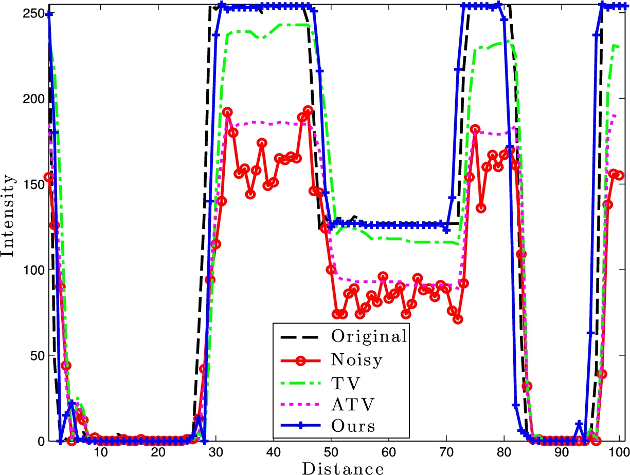
Fig. 3
One dimensional (1D) line taken across the original, noisy, and denoised results to show the denoising capabilities. Dashed ($--$) is the original (noise-free), dash-circled ($-\mathrm{o}-$) is input noisy signal, dash-dotted ($-.-$) is the TV, dotted (...) is the ATV, and solid line with plus ($-+-$) is our proposed approach.
In our first experiment we consider a synthetic
$Shapes$ image of size
$320\times 320$ pixels which consists of various objects with different scales and intensity values. To test different TV regularization filters we add Poisson noise of strength
$20\% $ to the original pristine image as shown in Fig.
2(a). Figure
2(b–d) show optimal restoration results (with respect to the highest MSSIM value) with TV (Le
et al.,
2007), adaptive TV with (
5), and our proposed adaptive TV with (
9). As can be seen in the bottom row of concentric circles (from the full
$Shapes$ image top right corner part), our proposed approach obtains better noise removal with edges preserved in all the objects. Moreover, compared to TV regularization we obtain no staircasing artifacts in flat regions. The slight smoothing of sharp corners is part of the TV regularization formulation and further corner adaptive weight in Eq. (
4) is required to preserve them. To see the denoising effects clearly, in Fig.
3 we show a cross section taken in Fig.
2 and their corresponding denoising results with TV regularization filters. As can be seen, our regularization obtains better edge preservation without staircasing artifacts in flat regions.
Table 1
Comparison of TV, ATV – adaptive TV with inverse gradient weight (
5) and Our – proposed generalized inverse gradient weight (
9) based regularizations on denoising standard test images with Poisson noise of strength
$20\% $. Smaller root mean squared error (RMSE), and (RE), and higher FOM, and MSSIM means better restoration capability. Best results for each image and for each error metric are in bold.
| Image |
Method |
RMSE |
RE |
FOM |
MSSIM |
| Lena |
TV |
0.4112 |
0.0548 |
0.9508 |
0.8230 |
|
ATV |
0.3637 |
0.0503 |
0.9667 |
0.8452 |
|
$k=0.0625$, $\lambda =8$
|
Our |
0.3532 |
0.0456 |
0.9708 |
0.9125 |
| Cameraman |
TV |
0.4681 |
0.0501 |
0.9752 |
0.7892 |
|
ATV |
0.3701 |
0.0443 |
0.9834 |
0.8216 |
|
$k=0.0555$, $\lambda =9$
|
Our |
0.3622 |
0.0418 |
0.9901 |
0.8993 |
| Boat |
TV |
0.4711 |
0.0534 |
0.9537 |
0.7397 |
|
ATV |
0.4388 |
0.0507 |
0.9618 |
0.8166 |
|
$k=0.0625$, $\lambda =12$
|
Our |
0.4197 |
0.0445 |
0.9693 |
0.8884 |
Table
1 shows error metrics values for restoring corrupted
Lena,
Cameraman and
Boat test images from the USC-SIPI Miscellaneous dataset. We fixed all the common parameters equal for the TV regularization variants and vary only the contrast parameter
k, and Lagrangian multiplier
λ, see Zhou and Lia (
2012).
3.3 X-Ray Imagery Comparison Results
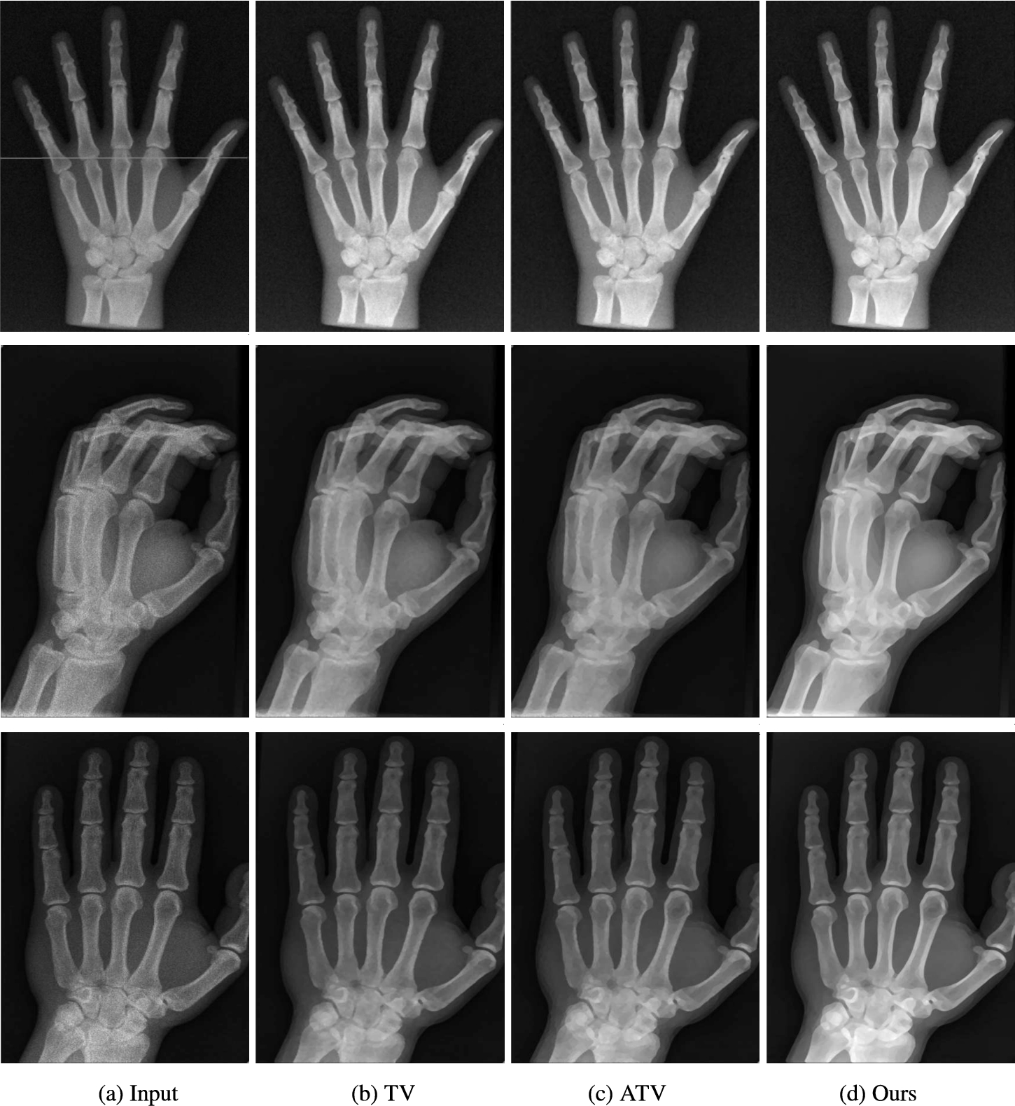
Fig. 4
Comparison of different regularization denoising filters and variational – PDE methods on X-ray images. (a) Input X-ray images. Restoration with (a) traditional TV, (b) adaptive TV with inverse gradient weight (
5), and (c) our proposed generalized inverse gradient weight (
9) based regularizations. Better viewed online and zoomed-in.
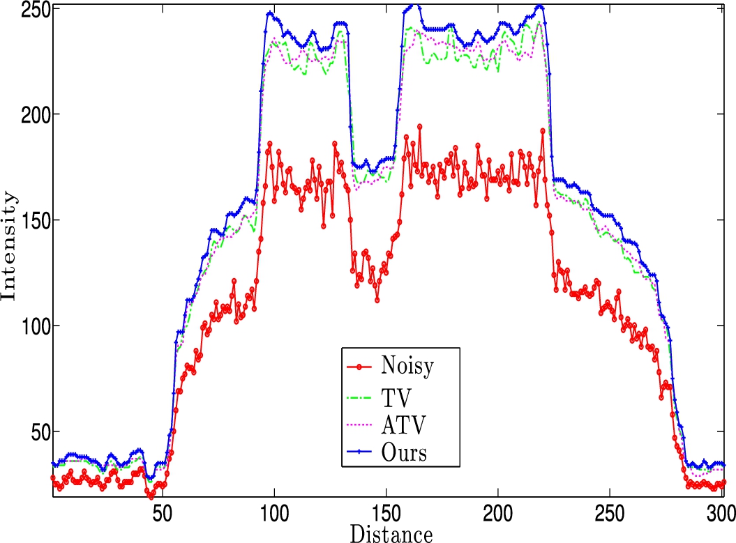
Fig. 5
One dimensional (1D) line taken across the original, noisy, and regularization results of X-ray image in Fig.
4(a) top, to show the denoising capabilities. Dash-circled (-o-) is input noisy signal, dash-dotted (-.-) is the TV, dotted (...) is the ATV, and solid line with plus (-+-) is our proposed approach. We show only one finger corresponding the left most.
Figure
4 shows comparison restoration results with TV, ATV, and our proposed regularization filters on different X-ray imagery of hands. Our proposed generalized inverse gradient weight based TV regularization obtains better edge preservation with overall pixel intensity improvement indicating that the signal dependent Poisson noise is removed effectively. To show the denoising clearly in Fig.
5 we show a line taken across from the X-ray image in Fig.
4(a) top and the corresponding results from Fig.
4(b–d). We only show the first finger on the left (300 pixels long). It is clear that our proposed regularization obtains better restoration of improved intensity profile (contrast enhanced) and without staircasing artifacts. In summary, we see that our proposed ATV regularization works well in preserving important details while removing noise effectively when compared with related denoising methods from the literature.
4 Conclusions
In this paper, we considered a localized inverse gradient weighted adaptive total variation regularization for removing quantum noise in X-ray imagery. By using local histograms along with gradient edge indicator function we obtain better roadmaps of discontinuities present in the image thereby better guiding the total variation regularization without creating blocky artifacts. Efficient dual minimization for total variation regularization with alternating direction method of multipliers optimization. Experimental results are given to highlight the applicability of our proposed approach along with comparison with other related denoising methods. Results indicate that we obtain better accuracy in terms of signal to noise ratio and structural similarity preservation.

