Abstract
Analysing massive amounts of data and extracting value from it has become key across different disciplines. As the amounts of data grow rapidly, current approaches for data analysis are no longer efficient. This is particularly true for clustering algorithms where distance calculations between pairs of points dominate overall time: the more data points are in the dataset, the bigger the share of time needed for distance calculations.
Crucial to the data analysis and clustering process, however, is that it is rarely straightforward: instead, parameters need to be determined and tuned first. Entirely accurate results are thus rarely needed and instead we can sacrifice little precision of the final result to accelerate the computation. In this paper we develop ADvaNCE, a new approach based on approximating DBSCAN. More specifically, we propose two measures to reduce distance calculation overhead and to consequently approximate DBSCAN: (1) locality sensitive hashing to approximate and speed up distance calculations and (2) representative point selection to reduce the number of distance calculations.
The experiments show that the resulting clustering algorithm is more scalable than the state-of-the-art as the datasets become bigger. Compared with the most recent approximation technique for DBSCAN, our approach is in general one order of magnitude faster (at most 30× in our experiments) as the size of the datasets increase.
1 Introduction
Unlocking the value in the masses of the data stored and available to us has become a primary concern. Medical data, banking data, shopping data and others are all analysed in great detail to find patterns, to classify behaviour or phenomena and to finally predict behaviour and progression. The outcome of these analyses is ultimately hoped to predict behaviour of customers, to increase sales in marketing (Chen
et al.,
1996), to optimize diagnostic tools in medicine, to detect disease earlier, to optimize medical treatments for a better outcome (Adaszewski
et al.,
2013; Venetis
et al.,
2015) and so on.
Generating insightful knowledge from data, however, is not efficient today. While there exists a plethora of tools and algorithms for the analysis and clustering of data, most of them have a considerable complexity, meaning they will not scale well to the massive datasets we see today. They are very efficient on the small datasets we dealt with until recently but as the amounts of data grow rapidly, these algorithms do not scale and fail to provide a fast analysis.
At the same time, data analysis rarely is a straightforward process. All clustering algorithms require the tuning of parameters, e.g. number of clusters in k-means, maximum distance (ϵ) in DBSCAN, etc., and also the data preparation process frequently needs to be repeated, for example, to adjust the level or aggregation or similar. Clearly, throughout the process of iteratively improving the analysis, the results need not be exact. Instead, by sacrificing little precision, we can substantially accelerate each analysis and thus the overall process.
More formally, the problem we address is density-based clustering, i.e. given a set of points P in d-dimensional space ${\mathbb{R}^{d}}$ (with typically a very high d), the goal is to group points into clusters, i.e. to divide the points into dense areas separated by sparse areas. Existing approaches generally differ in how dense and sparse areas are defined but all approaches share that distance calculations account for the majority of the execution time. By reducing the number of distance calculations and approximating the remaining ones, we can trade accuracy for efficiency and scalability.
In this paper we propose ADvaNCE (
Approximate
De
Nsity-Based
Clust
Ering) (Li
et al.,
2016), a novel approximation approach for DBSCAN, arguably the most prominent density-based clustering approach used today. Our approach reduces the overhead of calculating distances with two measures. First, we use locality sensitive hashing (LSH) to approximate each distance calculation and thus accelerate it. Clearly, this step in itself already introduces approximation. Second, we approximate the dataset by only retaining representative points which summarize its structure. Doing so reduces the number of points and consequently also the number of distance calculations. Like locality sensitive hashing, this measure approximates the result as well.
The resulting approach outperforms the classic DBSCAN by orders of magnitude by sacrificing the accuracy in the order of 0.001%. More importantly, ADvaNCE outperforms the state-of-the-art approximate DBSCAN approaches by at most 30×. It scales well with an increasing size of datasets for small ϵ’s and consistently outperforms the state of the art.
The remainder of this paper is structured as follows. In Section
2 we discuss in detail DBSCAN along with its known optimizations but also its challenges. We then move on to give an overview of ADvaNCE in Section
3 and discuss in more detail the approximate acceleration based on locality sensitive hashing in Section
4.2 and the approximation based on representative points in Section
5. To understand the benefits and limitations of ADvaNCE we first analyse it analytically in Section
6 and then compare ADvaNCE’s efficiency to related approaches in Section
7. We then analyse its performance in detail in Section
8. We discuss the state-of-the-art of clustering algorithms (approximate and exact) in Section
9 and finally draw conclusions in Section
10.
2 DBSCAN and Its Challenges
DBSCAN is arguably the most renowned density based clustering algorithm. We first give an overview of DBSCAN, present a first optimization and then motivate our approach with a motivation experiment.
2.1 DBSCAN Recap
DBSCAN is a density based clustering algorithm that takes two parameters ϵ and $\mathit{minPts}$ to determine what areas of the datasets are dense/sparse and finally to compute the clustering result. For every input point p, if the neighbourhood within radius ϵ contains at least $\mathit{minPts}$ number of points, we call point p a core point.
Definition 1.
Point
p is density reachable from point
q if there exists a sequence of points
${p_{1}},{p_{2}},{p_{3}},\dots ,{p_{n}}$ such that either:
-
1. ${p_{1}}=p$ and ${p_{n}}=q$;
-
2. ${p_{1}},{p_{2}},{p_{3}},\dots ,{p_{n-1}}$ are core points;
-
3. ${p_{i+1}}$ is in the neighbourhood of ${p_{i}}$ with radius ϵ.
Points that are not core points themselves but are density-reachable from any core point are called border points. A cluster defined by DBSCAN starts from a single core point and gradually adds all density-reachable points from any points in this cluster, which leads to a chain effect, and the cluster grows until it is finally complete. Points that are neither core points nor border points are called noise points and do not belong to any cluster.
2.2 Grid-Based Optimization
Naive implementations of the DBSCAN algorithm (Ester
et al.,
1996) compute distances between all pairs of data points in the dataset in
$O({n^{2}})$. A first proposed optimization uses a KD-Tree (Bentley,
1975) to reduce the number of distance calculations between data points.
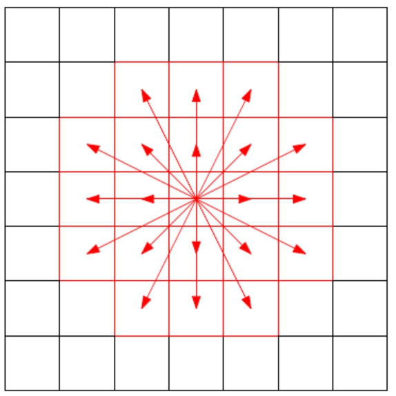
Fig. 1
Neighbouring cells of c are in red.
At the centre of ADvaNCE is a grid-based optimization (Gunawan,
2013) of DBSCAN that further reduces the distance calculations. The grid used has the same dimensions as all points in the dataset. With this grid we can considerably reduce the number of distance calculations: given a point
p, we only have to search in a fixed number of cells around
p to find other points within distance
ϵ of
p. More precisely, given the centre cell
c in which
p is located, we only have to search the cells
${c^{\prime }}$ with
$\mathit{dist}(c,{c^{\prime }})<\epsilon $, i.e. the neighbouring cells
$N(c)$ (red in Fig.
1).
The grid uses uniform spacing of the cells in all dimensions, making assignment of points to cells and related calculations straightforward. With the grid, the algorithm has four distinct phases.
Grid construction: in the assignment phase the algorithm iterates over all points and maps each point to the grid cell that encloses it. To eventually reduce the number of distance calculations, we choose the grid cell width as $\frac{\epsilon }{\sqrt{D}}$ with D as the dimension, guaranteeing that all points within a cell are by definition within distance ϵ of each other and thereby form a cluster.
Determining core points: the goal of this phase is to determine core points. For this phase the choice of grid cell width used in the first phase is crucial. As mentioned previously, if the grid cell width in the first phase is set to $\frac{\epsilon }{\sqrt{D}}$, then the diagonal of the cell is ϵ and consequently the distance between any two points in the same cell is at most ϵ. If a cell c contains more than $\mathit{minPts}$ points, all the points inside cell c are consequently core points.
Merge clusters: most important in this phase is that we consider each non-empty cell as a small cluster. Further, if two core points in two different cells are within distance less than ϵ of each other, these two points belong to the same cluster and the clusters need to be merged.
To compute all clusters, the optimization generates a graph $G=(V,E)$ where V represents all non-empty cells. Given two cells ${c_{1}}$ and ${c_{2}}$, E contains an edge between ${c_{1}}$ and ${c_{2}}$ if there exist core points ${p_{1}}$ in ${c_{1}}$ and ${p_{2}}$ in ${c_{2}}$ with $\mathit{dist}({p_{1}},{p_{2}})<\epsilon $. The result of the merge cluster phase consequently is the connected components of graph G which represent the clusters.
Determine border points: given a non-core point p in cell c (by definition a cell with less than $\mathit{minPts}$), we check all core points in neighbouring cells $N(c)$, and find the core point q with the minimum distance to p. Then p is a border point and belongs to the cluster of core point q. If there are no core points in $N(c)$, then p is a noise point and does not belong to any cluster.
2.3 DBSCAN Challenges
A considerable challenge of DBSCAN (and other clustering approaches) is the number of distance calculations and the time needed for them. Even for the optimized DBSCAN algorithm (Gunawan,
2013) the number of distance calculations is substantial. To make matters worse, the number grows rapidly with increasing dataset size.
We demonstrate this problem with a motivation experiment where we increase the size of the dataset from 0.125 millions to 1 million. The datasets used have five dimensions and are randomly generated (Gan and Tao,
2015). For DBSCAN we set the parameters to
$\epsilon =5000$ and the minimum number of points to 100 (Gan and Tao,
2015). We repeat the experiment for each dataset three times and report the average.
As the results in Fig.
2 show, the share of the total time needed to execute distance calculations in DBSCAN starts with a few seconds for a very small dataset of 125’000 and grows rapidly to a substantial share of more than 60% for a dataset of 1 million. Clearly, the share of the overall time spent on distance calculations is substantial and grows rapidly. As we will show in the remainder of this paper, we speed up DBSCAN considerably and enable it to scale by using approximation in two respects. First, we use approximation to reduce the total number of distance calculations, and second, we use approximation to accelerate the remaining distance calculations. As we will show, only little precision has to be sacrificed using ADvaNCE to accelerate the clustering process considerably.
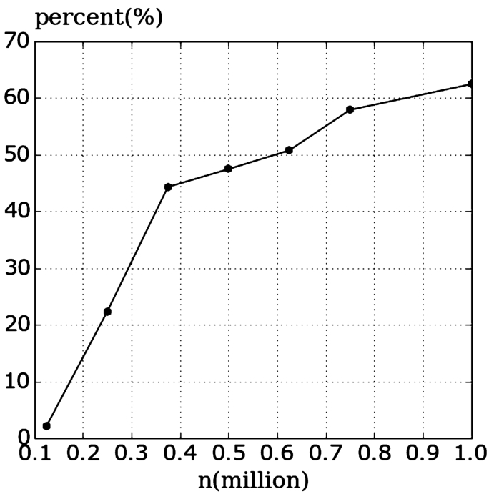
Fig. 2
Share of overall time needed for distance calculations.
3 ADvaNCE Overview
ADvaNCE uses the key insight that for large multi-dimensional datasets the time needed to find clusters is primarily driven by the number of distance computations needed. While in the previous work Gunawan (
2013) has substantially reduced this number, it is still considerable and grows rapidly for increasingly big datasets. By approximating the cluster computation in a grid-based DBSCAN (Gunawan,
2013) implementation we considerably accelerate the process.
The first approximation reduces the number of distance calculations, or more precisely, the number of neighbouring cells a cell has to speed up clustering. Using locality sensitive hashing (Andoni and Indyk,
2008) (LSH) we can approximate distances between the points and efficiently establish whether two points are within distance
ϵ of each other.
A second approximation reduces the points considered in each cell. To decide whether or not two grid cells, each containing more than $\mathit{minPts}$ and thus containing only core points, should be joined, not all points need to be considered. To obtain an approximate result it is sufficient to take into account primarily points closer to the border of the cell: if each of two cells has a point within distance ϵ of each other, then there is no need to test further points.
Particularly, the former optimization merges the cells with at least $\mathit{minPts}$ (which are consequently all core points) approximately and efficiently. It does, however, only join a subset of neighbouring cells at a time and consequently several iterations are needed to join all neighbouring cells of core points. ADvaNCE consequently is run iteratively to join cells. It runs iteratively until the result converges, i.e. until the result no longer changes between two iterations (set as a parameter).
4 ADvaNCE: Approximate Neighbourhood
While the basic Grid based algorithm is very efficient in two dimensions with $D=2$ and in case the width of each cell is set to $\frac{\sqrt[D]{\epsilon }}{2}$ (and the diagonal of each cell consequently is ϵ), in higher dimensions the number of $N(c)$ cells grows considerably. For example, in five dimensions the cell width becomes very small with $\epsilon /\sqrt{(}5)$, meaning that three cells need to be searched in each dimension and $N(c)$ thus contains ${7^{5}}$ cells. Merging cells into clusters will be very time consuming as all of $N(c)$ (${7^{5}}$ cells in five dimensions) has to be searched for every core point.
In the following we first discuss the basic concept of approximating the neighbourhood and then present how to design the algorithm that (a) approximates the neighbourhood and (b) clusters based on the approximation.
4.1 Using Locality Sensitive Hashing to Approximate
As discussed previously, searching in the neighbouring cells
$N(c)$ is crucial to the execution of grid-based DBSCAN (Gunawan,
2013) as it is an integral part of every step (except when constructing the grid). The number of cells in
$N(c)$, however, is growing uncontrollably with an increasing number of dimensions. The basic idea of our approximate algorithm is to find an approximate neighbour for each core point using locality sensitive hashing instead of searching in the potentially large number of cells in
$N(c)$. We consequently use the approximate neighbours to finish DBSCAN with a controllable precision.
In the context of ADvaNCE we use locality sensitive hashing (LSH, Andoni and Indyk (
2008)) to approximate and reduce the neighbourhood that needs to be considered. The LSH functions
H we use are random hyperplane projection functions. More precisely, given two points
$p,q$ in dimension
${D_{1}}$ (the dimension of the input data) we use
H a set of random hyperplane distance functions to project
p and
q into dimension
${D_{2}}$, thereby approximating the distance between them. With this, we can assert the following about the approximate distance between
p and
q:
-
1. If $\mathit{dist}(p,q)<\epsilon $, then for every function ${H_{i}}\in H$, we have ${H_{i}}(p)-{H_{i}}(q)<\epsilon $;
-
2. If $\mathit{dist}(p,q)>\epsilon $, then for every function ${H_{i}}\in H$, there is a considerable chance that ${H_{i}}(p)-{H_{i}}(q)>\epsilon $ and there is a small possibility that ${H_{i}}(p)-{H_{i}}(q)<\epsilon $.
With this we consequently can construct a new grid
$\mathit{NG}$ in
${D_{2}}$ with
$\mathit{cellWidth}=\epsilon $ and assign each point to the corresponding cell. Given a point
p, we define the cell
c in the new grid
$\mathit{NG}$ that contains
p as the approximate neighbour of
p, denoted by
$\mathit{AN}(p)$ and all points in
c will serve as approximate neighbour points of
p. The algorithm is shown in pseudocode in Algorithm
1.
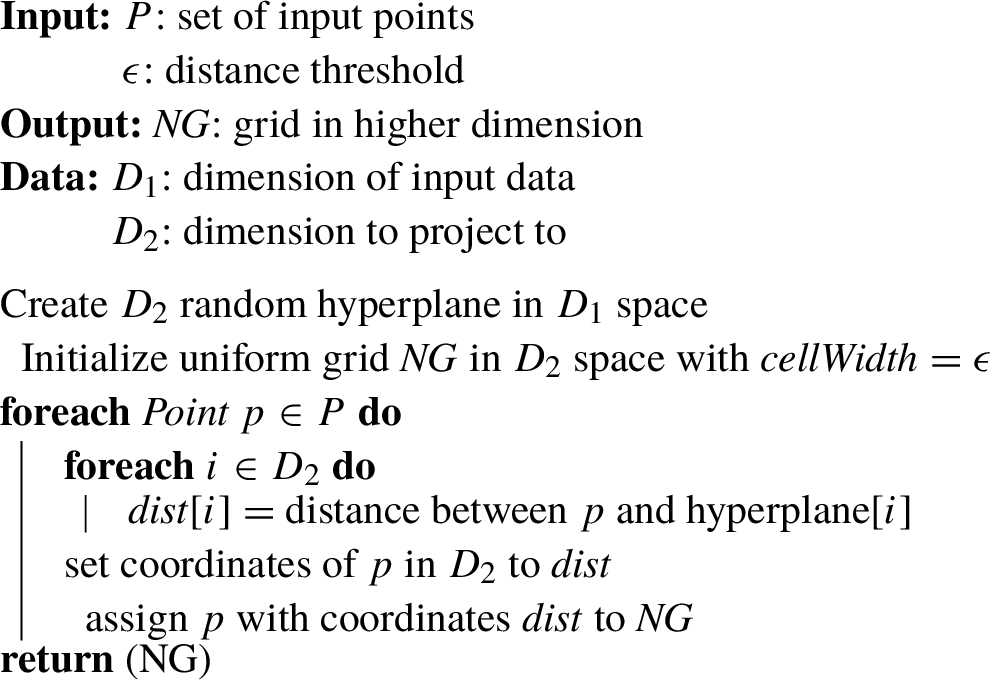
Algorithm 1:
HashAndAssign.
Given our approach to approximation, it is possible that points that are within the ϵ neighbour sphere $B(p,\epsilon )$ can not be found in a neighbour cell in $\mathit{NG}$ due to the approximation. In the grid $\mathit{NG}$ in ${D_{2}}$ space $B(p,\epsilon )$ may be split into two parts. We address this issue by iterating and accumulating the hashing results to obtain a good approximation of the true ϵ neighbours.
4.2 ADvaNCE-LSH – Approximate, LSH-Based DBSCAN
Using the approximate neighbours in
$\mathit{NG}$ generated based on locality sensitive hashing we propose ADvaNCE-LSH, our approximate grid-based DBSCAN algorithm using LSH as described in Andoni and Indyk (
2008). The functions we use are hashing functions with a
p-stable distribution (Andoni and Indyk,
2008). Independent of the dimensionality of the input data, we project to 8 dimensional space. An overview in pseudocode is given in Algorithm
2.
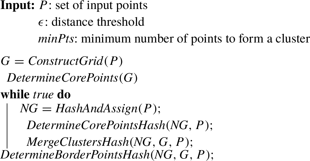
Algorithm 2:
ADvaNCE-LSH – approximate, LSH-based DBSCAN.
The $\mathit{Construct}$ $\mathit{Grid}$ and $\mathit{Determine}$ $\mathit{Core}$ $\mathit{Points}$ functions are very similar to the functions explained for the basic grid-based DBSCAN implementation. In this version we only mark the points as core points when the cell contains more than $\mathit{minPts}$ points and leave it to Determine Core Points Hash to determine which of the remaining points are core points.
The condition for the while loop in Algorithm
2 can be set to a fixed number of iterations. Alternatively, and to control the precision of the result better, we can use a heuristic termination condition that counts the number of core points or the number of clusters and stops when the accuracy no longer improves, i.e. when there is no more change between two iterations.
The function Determine Core Points Hash and Determine Border Points Hash are the approximate versions of Determine Core Points and Determine Border Points described previously. More precisely, in Determine Core Points Hash, for every non-core point p, we count the number of points in $\mathit{AN}(p)$ within ϵ of point p. Although $\mathit{AN}(p)$ is not equal to $B(p,\epsilon )$, we can converge to it through iterations. The accumulation of $\mathit{AN}(p)$ in successive iterations will converge to $B(p,\epsilon )$ and we can gradually compute the full result. In Determine Border Points Hash we find the nearest core point for every non-core points p in $\mathit{AN}(p)$ generated by LSH. This step can also be repeated several times to improve the accuracy.
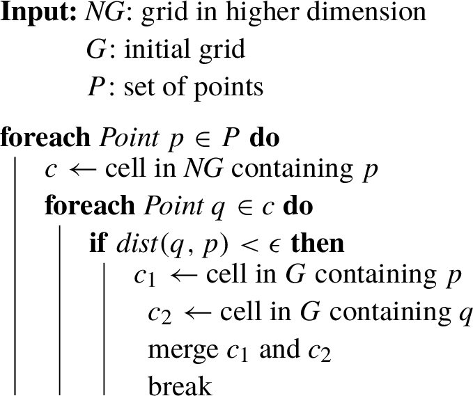
The function
Merge Clusters Hash is the approximate version of
Merge Clusters discussed previously. If two core points
p and
q are in the same cell in
$\mathit{NG}$ and their distance is less than
ϵ, the two small clusters that contain
p and
q are merged. The algorithm is illustrated in Algorithm
3.
Algorithm 3:
Approximate cluster merging.
In Algorithm
3 we merge the clusters in
${D_{1}}$ using the hashing result in
${D_{2}}$ space. Crucially, we add a break in the for-loop because we do not merge all possible clusters in one go but instead use a number of iterations to gradually merge the clusters and terminate when we meet the condition of the while loop in the main algorithm (Algorithm
2).
5 ADvaNCE: Representative Points Approximation
Given the basic approximation discussed before, we can further accelerate Grid-based DBSCAN featuring locality sensitive hashing called ADvaNCE-LSH. More particularly, in case of very dense datasets, the number of points in a cell that need to be compared to points in neighbouring cells is considerable, leading to substantial overhead. This leads to a bottleneck in the main iteration described previously as we have to iterate through all points in a cell and need to determine their relationship to points in neighbouring cells.
To address this issue we have designed a further optimization. Given $\mathit{minPts}$, which is the minimum number points to form a cluster, we set the maximum number of points in each cell to be $\mathit{maxNum}$ where $\mathit{maxNum}>\mathit{minPts}$ and ignore the other points in the main iteration.
For every cell c in the original grid G there are three cases:
-
1. If $|c|<\mathit{minPts}$, then we can not (yet) determine whether the points in c are core points and c is thus not affected by this approximation;
-
2. If $|c|\geqslant \mathit{minPts}$ and $|c|\leqslant \mathit{maxNum}$, then all points in c are core points and this cell will also not be affected by this approximation;
-
3. If $|c|>\mathit{maxNum}$, then it follows that $|c|>\mathit{minPts}$ and all points in c are core points. All points in c belong to the same cluster so we only need to identify which cluster this cell c belongs to during the main iteration. Although we ignore $|c|-\mathit{maxNum}$ points we can still determine which cluster they belong to.
Key to the approach is to choose $\mathit{maxNum}$ points such that we do not lose information (or at least can limit the information lost).
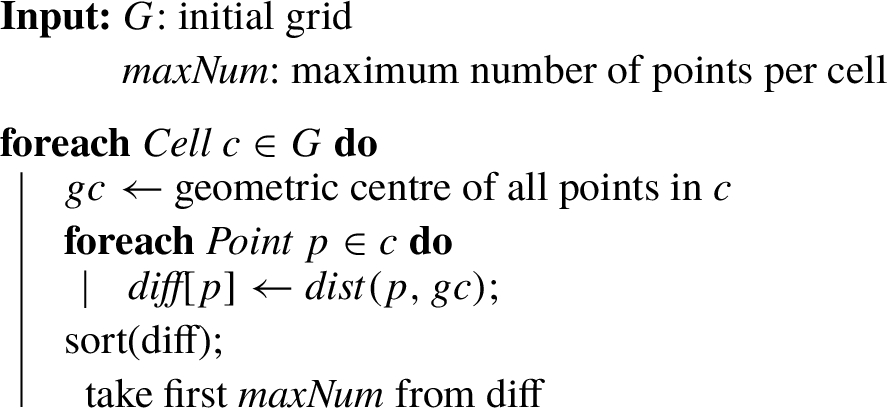
Using Algorithm
4 we select up to
$\mathit{maxNum}$ of the points that are near the border of each cell and in the
Merge Clusters Hash function we calculate the distance to determine the relationship between different cells. The points on the border of each cell are the most useful in determining what cells should be merged while the points near the centre of the cell are not very useful and we potentially ignore them. Consequently, Algorithm
4 will first calculate the geometric centre of all points and take the first
$\mathit{maxNum}$ points furthest away from the geometric centre.
Algorithm 4:
Reducing points in a cell.
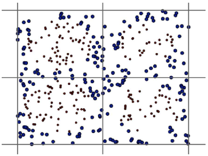
Fig. 3
Neighbouring cells of c in red.
To illustrate the algorithm we randomly generate 400 points in 4 cells and set the
$\mathit{maxNum}$ in each cell to be 50 and obtain the result in Fig.
3: the red-small points in the centre of each cell are points that are ignored by
Merge Clusters Hash algorithm while the big blue points around the border are still considered.
6 ADvaNCE: Analytical Analysis
To use ADvaNCE it is crucial to appreciate its benefits and to understand its limitations. In the following we therefore first analyse the accuracy of the algorithm and then reason about its time complexity.
6.1 Algorithm Accuracy
As ADvaNCE only approximates the DBSCAN result, it is of course crucial to analyse its accuracy. In the functions Determine CorePoints Hash and Merge Clusters Hash we use the approximate neighbours $\mathit{AN}(p)$ based on locality sensitive hashing instead of the actual ϵ neighbours $B(p,\epsilon )$. This may lead to a decreased accuracy in the following scenarios:
-
1. Given a point p, the number of points in $\mathit{AN}(p)$ is less than $\mathit{minPts}$, but $B(p,eps)$ has more than $\mathit{minPts}$ points. A core point p may therefore not be identified as core point in the current iteration;
-
2. Given cells ${c_{1}}$ and ${c_{2}}$, core points ${p_{1}}\in {c_{1}}$, ${p_{2}}\in {c_{2}}$ and $\mathit{dist}(p1,p2)<\epsilon $, but ${p_{1}}$ and ${p_{2}}$ are not in the same bucket after locality sensitive hashing. The two cells that should be merged may not be merged in the current iteration.
In both scenarios, merging of clusters or identification of core points may not occur. Crucial to ADvaNCE, however, is that it merges clusters in multiple iterations. As the number of iterations grows ADvaNCE will gradually determine more core points and merge more clusters that need to be merged. The impact of these two scenarios on the accuracy will consequently decrease monotonically and the algorithm will converge depending on the stop criteria which is either a fixed number of iterations or no change (in clusters or core points) in the last iterations.
Also note that we still perform distance calculations for points in $\mathit{AN}(p)$ to select the points that are truly in $B(p,\epsilon )$ and use these points to determine core points or merge clusters. We can therefore rule out the following two cases to occur in ADvaNCE:
In conclusion, the accuracy of ADvaNCE will increase monotonically with the number of iterations and an excessive number of iterations therefore cannot adversely affect the accuracy.
6.2 Time Complexity
The most time consuming part of ADvaNCE is the iterations of hashing and merging. In the following we thus analyse the time complexity of each iteration of ADvaNCE. Since Determine Core Points Hash and Merge Clusters Hash perform a linear search in the approximate neighbourhood $\mathit{AN}(p)$, the expected size of the $\mathit{AN}$, which is also the expected number of collisions for each query point in locality sensitive hashing, is the key to determining the running time of each iteration. We first discuss characteristics of level-i cells (number and distance between them) and the p-stable hashing functions used (probability of collision) before we reason about the time complexity.
Level-$\boldsymbol{i}$ cell characteristics: let P be the set of points in ${\mathbb{R}^{d}}$ where d is a constant (dimensions) and we construct the original grid G for all points in P. We start by defining level-i cells.
Definition 2.
Level-$\boldsymbol{i}$ cells: For a point q we find the cell c in G that contains q. Cells that are directly connected to c are level-0 cells. For level-i cells, the outer cells that directly connect to level-i cells are level-$(i+1)$ cells.
An example of level-
i cells in a 2D grid is shown in Fig.
4. Relative to the red cell, the yellow cells are level-0 cells, the green cells are level-1 cells, etc. The number of level-
i cells
${N_{i}}$ is
For every point
q in level-
i cells, the minimum distance between
q and
p,
${M_{i}}$ is
The maximum number of points in level-
i cell is a constant
$\mathit{maxNum}$ as we discussed in the context of the representative points approximation.
Hashing functions characteristics: if
${f_{p}}(t)$ is the probability density function of the absolute value of the
p-stable distribution, then for two vectors
${v_{1}}$,
${v_{2}}$ and with
$c=\| {v_{1}}-{v_{2}}\| $, the probability of collision
$p(c)$ is:
where
a,
b and
r are parameters for
p-stable LSH functions. In order to get a desirable hash result, we can also concatenate
k functions
h in
H and redefine the hash function as
$g(v)={h_{1}}(v),{h_{2}}(v),\dots ,{h_{k}}(v)$. In this case, the probability of collision
$p(c)$ is as follows:
With
p (the possibility function defined by a
p-stable LSH) and
k (the number of hash functions used) the number of collisions for a query point
q then is:
where
${p^{k}}(\| q-x\| )$ is the possibility of collision if two points with distance
$\| q-x\| $ and
D is the size of the dataset.
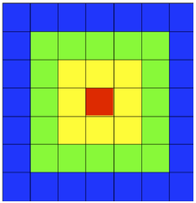
Fig. 4
Cells neighbouring the red cell are level-0 cells.
Time complexityanalysis: since we divide the whole dataset into cells of levels, we can redefine the number of collision by level-
i cells. In order to determine an upper bound for the number of collisions, we can assume that all points in level-
i cells have the distance
${M_{i}}$, which is the minimum distance they can have.
The expected number of collisions is proportional to an infinite series of
i. Given any
d (the dimension of the input data) we can always find
$k\geqslant (d+1)$ and the infinite series of
i will consequently converge to a constant regardless of how big
i is. The expected number of collisions can be expressed by the following function, where
C is a constant independent of the size of the dataset:
The expected size of the approximate neighbour $\mathit{AN}(p)$ therefore is $O(1)$. In function Determine Core Point Hash and Merge Clusters Hash, we perform a linear search in AN for every point, making the time complexity $O(n)$. Also, the hashing process itself is $O(n)$ and so the time complexity of one whole iteration consequently is $O(n)$.
7 Experimental Evaluation
In this section we first describe the experimental setup and then we perform a sensitivity analysis using synthetic datasets to understand the performance by changing one workload variable at a time. To demonstrate the benefits of our approach we also use real world datasets. Before we conclude we also analyse our algorithm in depth by discussing a breakdown of its performance.
7.1 Experimental Setup
The experiments are run on a Linux Ubuntu 2.6 machine equipped with Intel(R) Xeon(R) CPU E5-2640 0 CPUs running at 2.5 GHz, with 64 KB L1, 256 KB L2 and 12 MB L3 cache and 8 GB RAM at 1333 MHz. The storage consists of 2 SAS disks of 300 GB capacity each. Storage, however, is only used once to read the data into memory. In the following we discuss the software setup as well as the configuration details.
7.2 Software Setup and Datasets
We compare our algorithm against the most recent approximate DBSCAN implementation,
ρ-approximate DBSCAN available and set
ρ to 0.001 as recommended (Gan and Tao,
2015). We use two different versions of our approach, the first using the hashing approximation only (ADvaNCE-LSH) and the second using the representative point reduction as well (ADvaNCE). Crucially, the stop criteria for ADvaNCE (for both versions) is set so that it achieves the same accuracy as
ρ-approximate DBSCAN. Our approach is configured to use eight
p-stable hashing functions and convergence stops once no more clusters are merged.
Each algorithm implemented uses a single CPU core to ensure a fair comparison. Our approach is written in C++ while we use the executable provided for Gan and Tao (
2015). All implementations are compiled using g++ with -o3.
All experiments are repeated five times and the execution time is averaged.
We use the same synthetic datasets as in Gan and Tao (
2015) defined with a dimensionality
d, a restart probability
${\rho _{\mathit{restart}}}$, a target cardinality and a noise percentage
${\rho _{\mathit{noise}}}$. The datasets are generated using a random walk: the walk moves step by step a distance of
${r_{\mathit{shift}}}$ towards a random direction every
c number of steps. In each step, with probability
${\rho _{\mathit{restart}}}$, the walker restarts by jumping to a random location in the data space, resetting the step counter to
c. No matter if a restart has happened, the walker produces a point uniformly at random in the ball centred at its current location with radius 100. We repeat a total of
$n\times (1-{\rho _{\mathit{noise}}})$ steps generating the same number of points and add
$n\times {\rho _{\mathit{noise}}}$ uniformly distributed noise points. Put simply, we start to generate a cluster and in every step, with probability
${\rho _{\mathit{restart}}}$, start to generate a new cluster.
We also use two real datasets (Bache and Lichman,
2013): the
Household dataset in 7D as well as the
KDD Cup ’99 dataset (after PCA on the attributes) in 9D. The
Household dataset measures electric power consumption in one household with a one-minute sampling rate over a period of almost 4 years resulting in 2’049’280 data points. The
KDD Cup ’99 dataset consists of 4’898’431 data points representing detected network intrusion events.
All data is normalized in a domain of [0, 10’000] in all dimensions.
7.3 Accuracy Metric
To measure the accuracy of the approximate result we compare it to the exact result. We use the established omega-index to measure the quality of the clustering result (Collins and Dent,
1988; Murray
et al.,
2012). The omega-index assesses the similarity of two clustering results as the ratio of consistent pairs of points, i.e. a point
p needs to be in the same clusters in both clustering results. We compare the exact result obtained with the grid-based DBSCAN algorithm with either version of ADvaNCE. A value of the omega-index of 100% consequently means ADvaNCE’s result is precise and all values below that indicate how much the approximate result deviates from the precise result.
7.4 Synthetic Data
The synthetic datasets we use are generated as described previously. The DBSCAN parameter
$\mathit{minPts}$ is set to 100 (Gan and Tao,
2015).
$\mathit{maxNum}$ for the representative points approximation is set to
$\sqrt{\mathit{minPts}\times M}$ where
M is the maximum points per cell.
7.4.1 Increasing Dataset Size
In this first experiment we compare the execution time of our approach (both optimizations) with the most recent DBSCAN approximation technique. We cannot compare it with a basic, accurate DBSCAN as this takes too long to execute but infer from experiments that the exact DBSCAN implementation (Ester
et al.,
1996) is slower than
ρ-approximate DBSCAN (Gan and Tao,
2015). We execute the experiment in 5, 7, and 9 dimensions, increase the data points from 100’000 to 10 millions and set
ϵ to 5000.
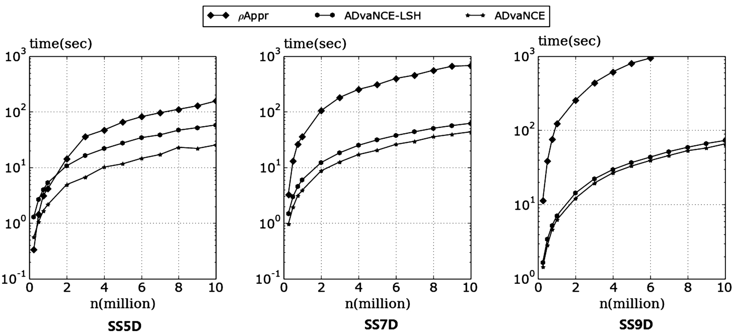
Fig. 5
Average execution time for experiments in 5, 7 and 9 dimensions with increasing dataset size.
As can be seen in Fig.
5, our approach using both approximations (ADvaNCE) outperforms
ρ-approximate DBSCAN (Gan and Tao,
2015) consistently and up to
$100\times $ (for 9 dimensions). As the number of dimensions increases, the execution time of
ρ-approximate DBSCAN grows. Our approach, on the other hand, shows consistent performance and improves execution time with an increase in the number of dimensions. This is because approximation by hashing works particularly well in higher dimensions. Overall our approach scales better with an increasing number of points in the dataset.
The gap between the two versions of our approach, ADvaNCE-LSH and ADvaNCE narrows as the number of dimensions grows. This effect can be attributed to hash-based approximation improving with an increasing dimensionality. As a consequence, the relative contribution of the representative points approximation shrinks and does not improve the result considerably for higher dimensions.
In Fig.
6 we measure the number of distance calculations instead of the execution time for the Grid-based DBSCAN implementation as well as both versions of ADvaNCE (we cannot measure it for
ρ-approximate DBSCAN as we only have access to the executable). Given the considerable execution time of analysing and measuring the number of distance calculations, we only measure the number of distance calculations from 0.2 to 1.6 million data points. Comparing the trends of the number of distance calculations as well as of the execution time in Fig.
5, we can see they have a similar shape which clearly indicates that the number of distance calculations is indeed the major contributor to the overall execution time.
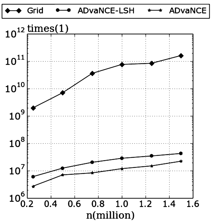
Fig. 6
Number of distance calculations with increasing dataset size.
7.4.2 Increasing Epsilon
In a next experiment we compare the approaches with increasing ϵ ranging from 5’000 to 50’000. Also here the basic, precise DBSCAN version takes too long to execute, we cannot include it in the results and consequently only compare ADvaNCE with ρ-approximate DBSCAN.
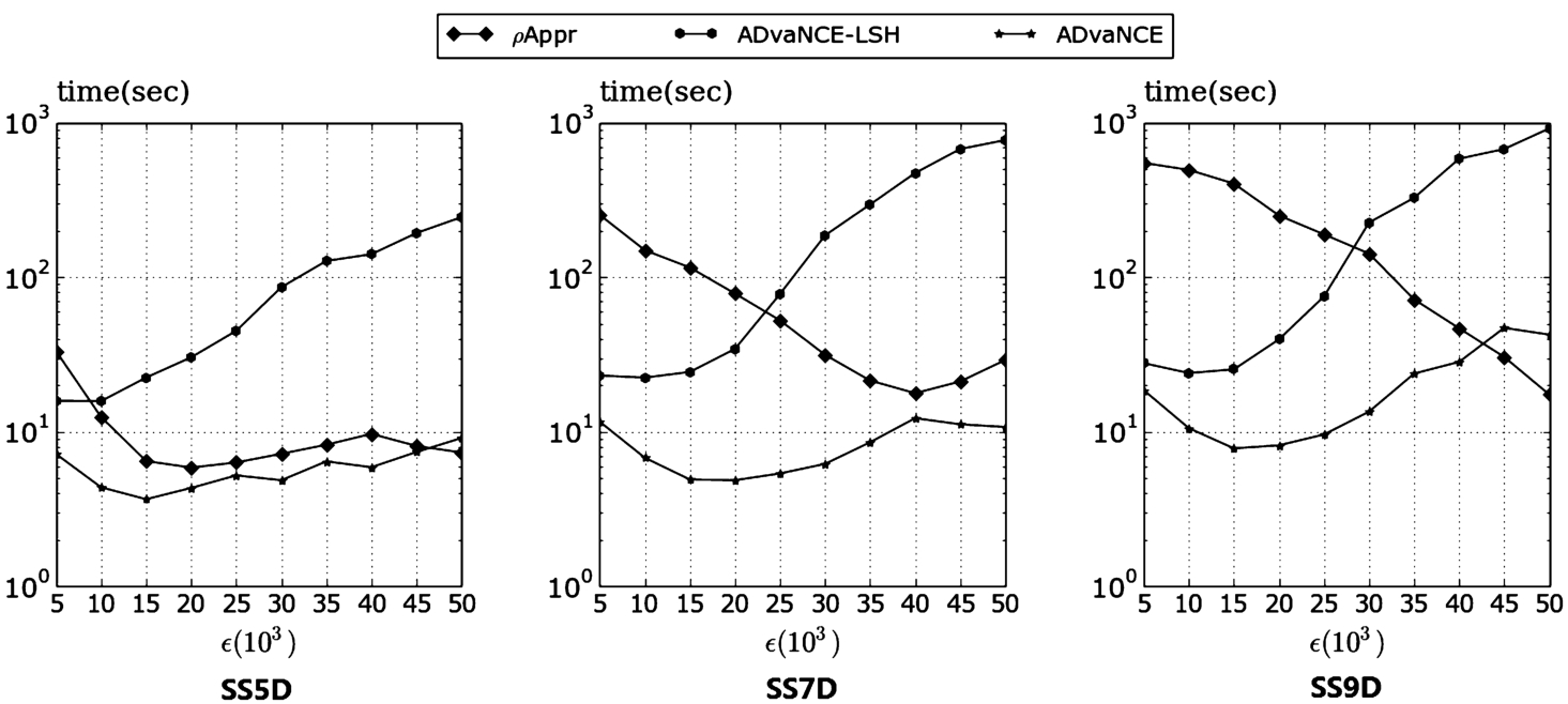
Fig. 7
Average execution time for experiments in 5, 7 and 9 dimensions with increasing ϵ.
As the results in Fig.
7 show, for an increasing
ϵ the performance of
ρ-approximate DBSCAN improves at first but then grows again (as can be seen in the experiment for five dimensions). Our approach based on hashing alone does not perform well as its execution time grows very rapidly. The problem with using hashing to compute distance calculations is that the precision degrades the bigger the
ϵ grows. Using the representative point approximation as well, however, again reduces the execution time considerably, to the point where it again outperforms
ρ-approximate DBSCAN.
For a very big ϵ (which is rarely used in real clustering applications), however, the ρ-approximate DBSCAN outperforms ADvaNCE. This effect is due to the dataset rather than the algorithm. As outlined previously, the data points are normalized to an interval of [0, 10’000] in all dimensions. In these experiments, however, the ϵ finally grows to 50’000 and, for example, in 5D the cell width is almost 23’000, resulting in only 5 cells in each dimension. With this few cells ADvaNCE cannot considerably reduce the number of distance calculations.
7.4.3 Increasing Dimensions
We also test the performance, i.e. execution time of our approach with an increasing number of dimensions (beyond 9 dimensions) and compare it with ρ-approximate DBSCAN. As we increase the dimension, we fix the remaining parameters: we use a synthetic dataset with three million data points and an ϵ of 5’000.
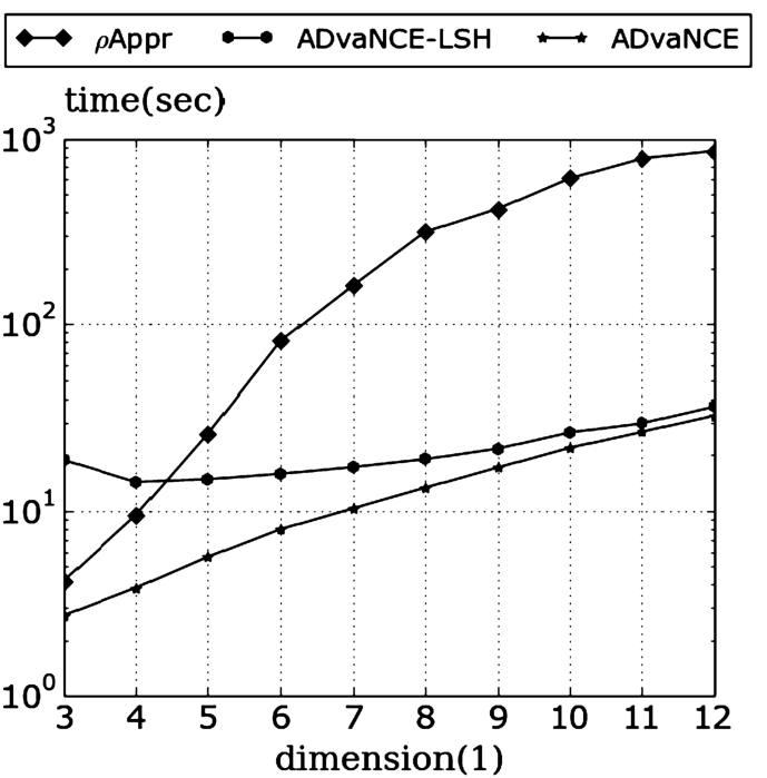
Fig. 8
Average execution time for experiments with an increasing number of dimensions.
As the result in Fig.
8 shows, although concave down and appearing to converge, the execution time of
ρ-approximate DBSCAN grows faster than the one of both ADvaNCE versions, resulting in a speed up of more than 10× for the biggest dimension tested.
The inaccuracy LSH introduces grows with the number of dimensions of the input data. As our results show, however, the impact of this effect is minimal in the experiments we carried out.
Also here, the relative difference between the two versions of ADvaNCE indicates that the higher the dimension, the more the hashing approximation contributes to the result of the execution time reduction thanks to the fact that the representative points approximation diminishes with increasing dimensionality. Towards the biggest number of dimensions tested, the execution time for ρ-approximate DBSCAN and our approach are parallel with ADvaNCE still outperforming the state-of-the-art by more than 10×.
The results in Fig.
9 show a similar picture. In this experiment we measure the number of distance calculations needed for an increasing number of dimensions for the same experimental setup. As the results show, the trend in both curves is the same as for the execution time in Fig.
8 and consequently the number of distance calculations is indeed what drives the execution time.
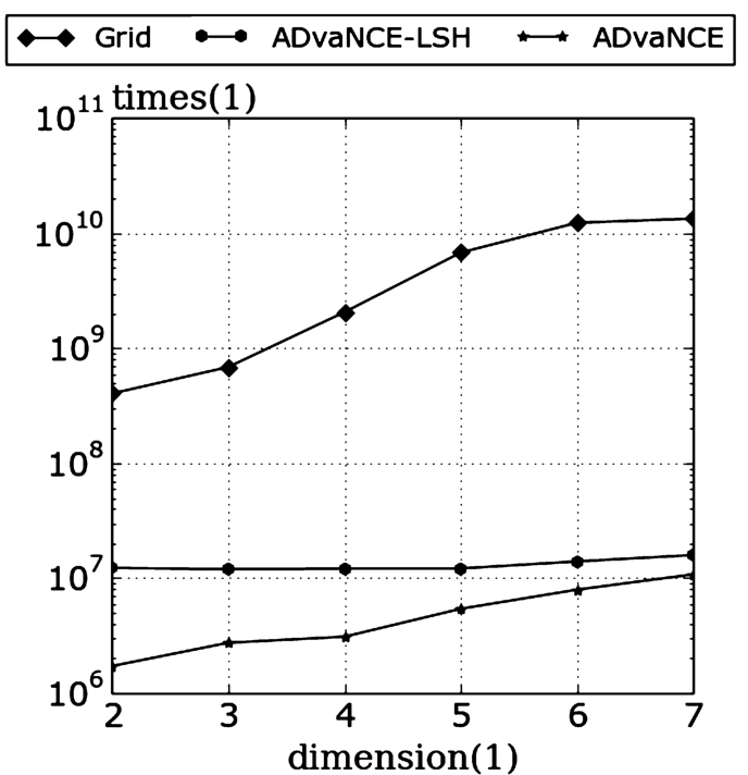
Fig. 9
Number of distance calculations with an increasing number of dimensions.
7.5 Real World Datasets
As a final litmus test of the overall execution time of ADvaNCE, we also compare it against
ρ-approximate DBSCAN on real world data. More specifically, we execute ADvaNCE and
ρ-approximate DBSCAN on the
KDD cup ’99 dataset as well as on the
Household dataset (Bache and Lichman,
2013). Given that the number of points per cell is very unbalanced in the real world datasets, we set
$\mathit{maxNum}$ for the representative approximation to
$\sqrt{A}\times M$ where
M is the maximum number of points in a cell and
A is the average number of points per cell.
As the results in Fig.
10 show, ADvaNCE generally outperforms
ρ-approximate DBSCAN. As we have already seen on the synthetic data, the ADvaNCE version which also features the representative points approximation further improves the efficiency and in general improves execution time by a factor of 5×. Interestingly, for the
KDD cup ’99 data the trend both versions of ADvaNCE exhibit is similar to
ρ-approximate DBSCAN but ADvaNCE is still 10x faster. For the
Household dataset both versions of ADvaNCE scale substantially better compared to
ρ-approximate DBSCAN: the execution time of
ρ-approximate DBSCAN grows very fast while ADvaNCE stays nearly flat.
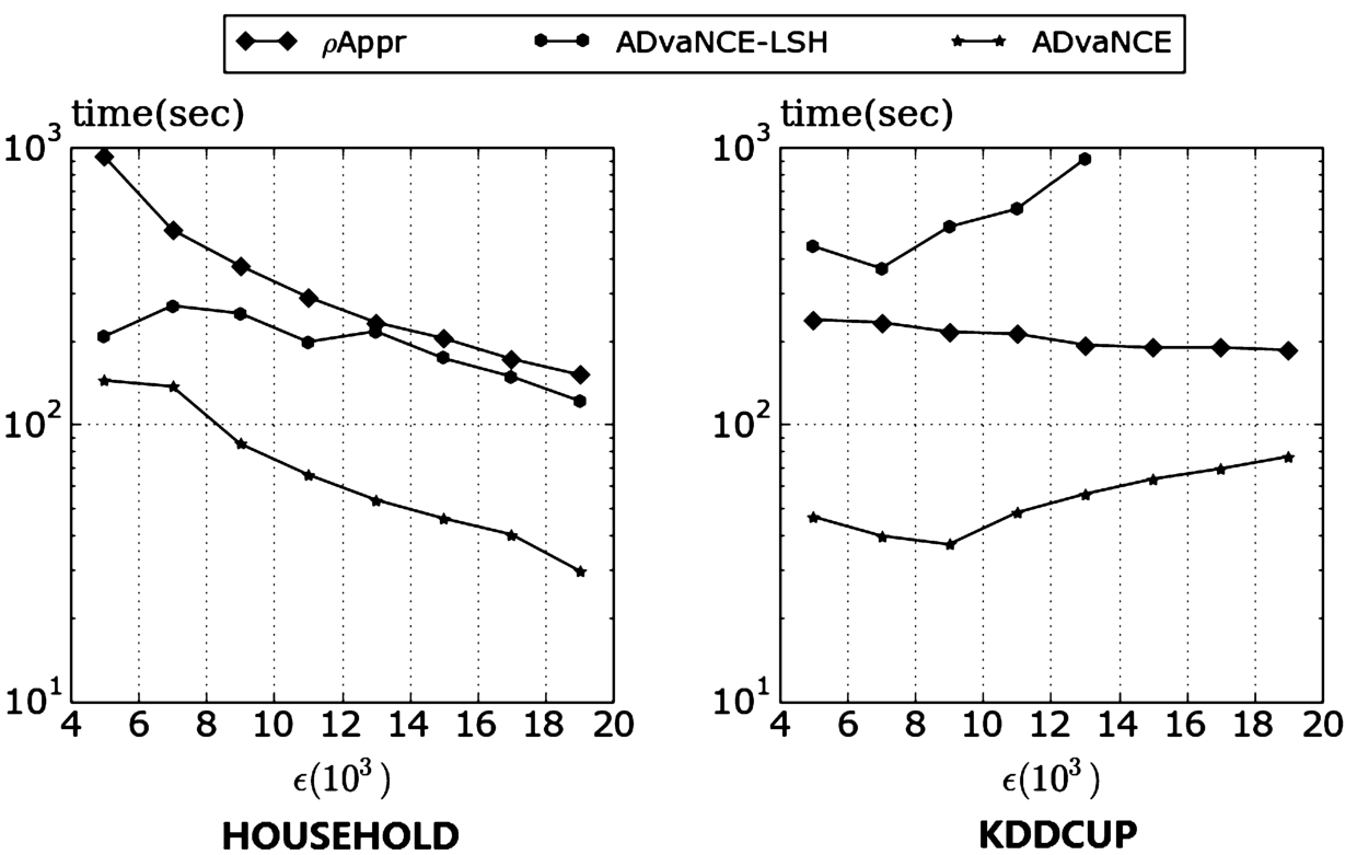
Fig. 10
Average execution time for experiments on real data with increasing epsilon.
In a next experiment we measure the execution time on the same real world datasets but we increase the size of the datasets. More precisely, we start with a tenth of the dataset and then increase it until we arrive at their full size.
As the results in Fig.
11 show, ADvaNCE also outperforms
ρ-approximate DBSCAN by more than a factor of 10. The trends are similar, but for an increasing dataset size, ADvaNCE has an edge over ADvaNCE-LSH as the gap between the trends grows bigger.
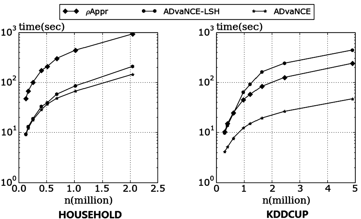
Fig. 11
Average execution time for experiments on real data with increasing dataset size.
8 In-Depth Analysis
Crucial to understanding the benefits of ADvaNCE is to analyse its behaviour in detail. In the following we thus first analyse the impact of increasing dimension and ϵ on the number of points (and thus execution time) and further analyse ADvaNCE through a breakdown of the execution time.
8.1 Number of Representative Points
As the dimension grows bigger, the maximum number of points and the average number of points in each cell is getting smaller (because the size of the cell is getting smaller:
$\mathit{cellWidth}=\frac{\epsilon }{\sqrt{(}d)}$ and because there are more directions to spread the data). Fig.
12 confirms this by measuring the maximum as well as average number of points per cell for an increasing number of dimensions. Consequently, ADvaNCE will perform well for an increasing number of dimensions even if only ADvaNCE-LSH, the version which does not curb the number of points per cell, is used.
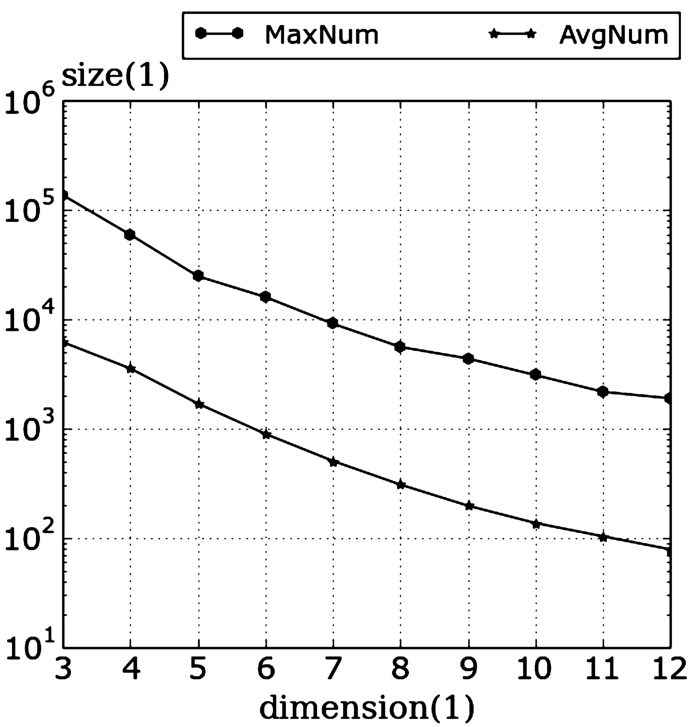
Fig. 12
Maximum and average number of points per cell for increasing dimensions.
For an increasing
ϵ the picture is different as Fig.
13 shows. In this experiment we measure the maximum (
Max Num), the average (
Avg Num) as well as the reduced number (
Redu Num) of points ADvaNCE considers. The reduced number of points is determined based on the maximum number of points in a cell
M and
$\mathit{minPts}$ as follows:
$\sqrt{\mathit{minPts}\times M}$.
The results clearly show that as ϵ grows bigger, the size of cell grows and the number of points in each cell grows as well. The number of points in each cell, however, is unbalanced: some cells contain a very large number of points while others contain only few. The second optimization of ADvaNCE, representative points, effectively addresses this by reducing the number of points considered (while only sacrificing little accuracy).
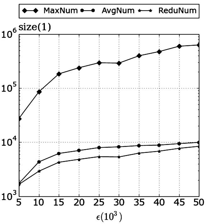
Fig. 13
Maximum, average and reduced number of points per cell for a growing ϵ.
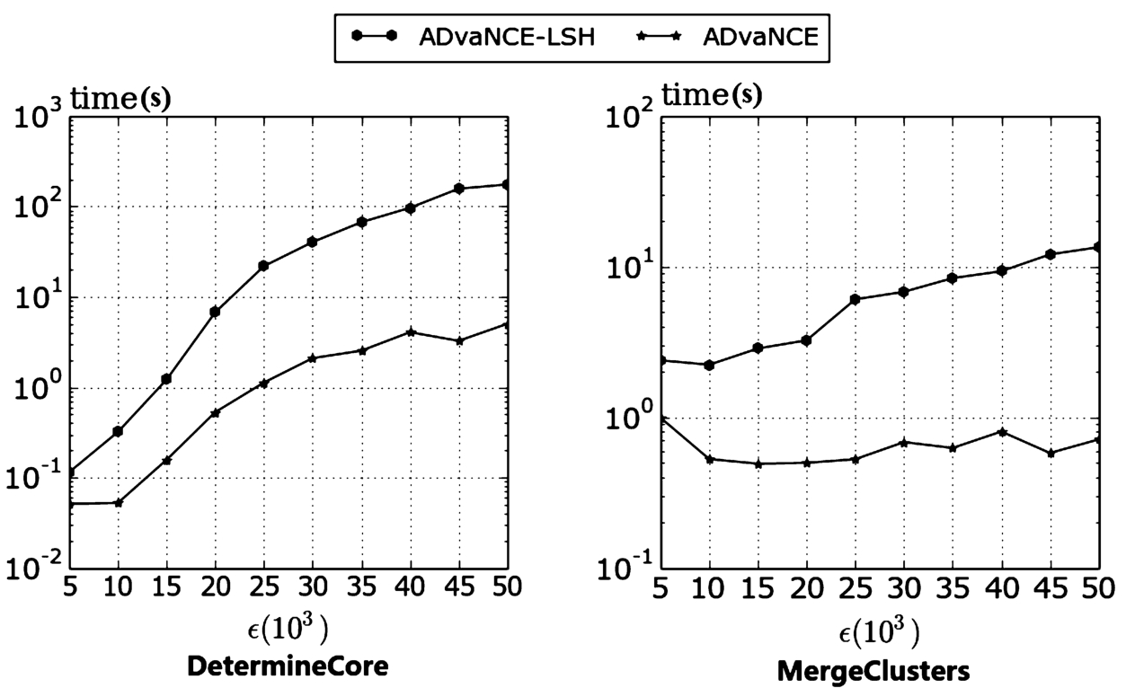
Fig. 14
Breakdown of the execution time of ADvaNCE.
8.2 Algorithm Breakdown
To understand the behaviour of ADvaNCE, we analyse the performance of its major building blocks
Determine Core Point LSH and
Merge Clusters LSH in the main iteration of our algorithm. We analyse the behaviour for an increasing
ϵ. As the results in Fig.
14 (left) show, if we only use ADvaNCE-LSH (i.e. ADvaNCE without the representative points approximation) as
ϵ grows, the time for determining core points will increase considerably from less than 0.1 s to more than 100 s. This is because in this step, for every non-core point, we have to search for all points in the approximate neighbourhood to see if this point is a core point. As
ϵ grows larger, the number of points in the approximate neighbourhood grows substantially and the time of this step will become the bottleneck. If we limit the number of points in each cell by the representative points approximation, however, the execution time is curbed.
As Fig.
14 (right) shows, as
ϵ grows, if we only use the hashing algorithm but do not limit the number of points, the time for
Merge Clusters LSH also increases. The increase, however, is moderate, going from less than 1 second to 10 seconds. This is because in this step we only find one core point in the approximate neighbourhood and then merge cells for every point. As
ϵ grows bigger, the number of points in the approximate neighbourhood also grows, but the time of this step consequently does not change substantially. If we limit the number of points in each cell to the representative number of points, the execution time of this step remains the same.
Assessing the execution time of these two functions, we see that if we only use ADvaNCE-LSH, the execution time will increase as ϵ grows, mainly because of the time spent on Determine Core Points. The execution time of both optimizations we use in ADvaNCE, however, remains almost the same (growing slightly) for an increasing ϵ thanks to the representative points approximation.
9 Related Work
In the discussion of related work we first give a brief overview of exact density-based clustering approaches before we move on to discuss in more detail the approximate algorithms devised.
9.1 Exact Approaches
Arguably the most renowned density based clustering approach is DBSCAN (Ester
et al.,
1996) itself. Given a set of points in typically high-dimensional space, it groups together points that are closely packed together (points with many nearby neighbours), marking as outliers points that lie alone in sparse regions. More formally, DBSCAN takes parameters
ϵ,
$\mathit{minPts}$ and identifies core points (points with at least
$\mathit{minPts}$ within radius
ϵ). DBSCAN then assigns core points within distance
ϵ of each other (along with non-core points within distance
ϵ) to a cluster. All other points are noise. DBSCAN can efficiently partition dense and sparse space but cannot deal well with varying density.
OPTICS (Ankerst
et al.,
1999; Breunig
et al.,
1999) addresses this issue of DBSCAN. Instead of using a fixed distance predicate,
ϵ is only used as a maximum distance and the distance is set in different areas of the dataset such that clusters can also be identified in areas of varying densities.
9.2 Approximate Approaches
More important to put our work in context, several approximate DBSCAN algorithms have also been devised in recent years.
ADBSCAN (Yeganeh
et al.,
2009) approaches the problem of accelerating the clustering of DBSCAN by reducing the number of region queries needed. The approach is based on the assumption that clusters are discovered by executing range queries on the dataset. It consequently tries to minimize the number of range queries. To do so, it defines skeletal points as the minimum number of points where range queries (with radius
ϵ) need to be executed to capture all clusters. The problem of finding the skeletal points is NP-complete and the ADBSCAN thus essentially proposes how to approximate the set of skeletal points using a genetic algorithm. By approximating the skeletal points, of course, the result of the clustering computation is approximate as well.
IDBSCAN (Borah and Bhattacharyya,
2004) works similarly and approximates and thus accelerates DBSCAN by reducing the range or neighbourhood queries needed. Instead of executing a query for all points in the vicinity of a core point, IDBSCAN only samples the neighourbood and executes a query on a subset of the points. To do so, the neighbourhood of a core point is partitioned into quadrants and a range query is only executed for the points in quadrants randomly chosen. The speed up achieved reaches a factor of six for the datasets tested. However, no guarantees about the results can be made.
l-DBSCAN (Viswanath and Pinkesh,
2006) uses the concept of
leaders to accelerate clustering. Leaders are a concise but approximate representation of the patterns in the dataset. l-DBSCAN on a first level clusters the leaders instead of the full dataset thereby accelerating the process. In a second step it replaces the leaders with the actual points from the dataset. With this process l-DBSCAN outperforms the precise version of DBSCAN by a factor of at most two.
ρ-approximate DBSCAN (Gan and Tao,
2015) guarantees the result of its clustering to be between the exact result of DBSCAN with (
$\epsilon ,\mathit{minPts}$) and (
$\epsilon \times (1+\rho ),\mathit{minPts}$). The approximation comes with a substantial speed up and scalability:
ρ-approximate DBSCAN is proven to run in
$O(n)$. The approach accomplishes this by using a grid approach where data points are assigned to a grid with cell width
$\frac{\epsilon }{\sqrt{d}}$. For an exact result the algorithm has to connect/combine all pairs of cells
${c_{1}}$,
${c_{2}}$ that (a) contain at least
$\mathit{minPts}$ and (b) contain two points (
${p_{1}}\in {c_{1}}$ and
${p_{2}}\in {c_{2}}$) within the distance of each other
ϵ. This problem is known as the biochromatic closest pair (BCP) and solving it precisely is exceedingly costly. However, solving BCP approximately (in
$\epsilon \times (1+\rho )$) can be accomplished in linear time. Clearly, the main benefit of this approach are the proven and firm theoretical bounds on error/approximation as well as the execution time.
Pardicle (Patwary
et al.,
2014) approximates DBSCAN in a supercomputing environment. It accelerates the basic DBSCAN approach by parallelization: after partitioning the multi-dimensional dataset into contiguous chunks, DBSCAN finds clusters in each chunk in parallel on different CPUs/cores of the supercomputing infrastructure. To account for clusters that span several chunks (analysed independently and in parallel on different cores), Pardicle replicates the border (of width
ϵ) of a chunk and copies it to adjacent chunks, i.e. to cores in the supercomputer. Doing so in essence makes the chunks overlap but also ensures correctness of the result. To reduce the overhead in terms of replication and distance calculations, not the exact border is calculated but it is sampled. Doing so approximates the results: the result in each chunk is accurate, but merging of clusters between adjacent chunks may fail.
10 Conclusions
In this paper, we develop ADvaNCE, a novel approach for approximating density-based clustering. ADvaNCE builds on a Grid-based optimization of DBSCAN and uses two approximations to accelerate and enable scalability of the clustering process. Understanding that distance calculations are the major contributor to the execution time of DBSCAN, ADvaNCE accelerates clustering by (a) approximating distance calculations and (b) reducing the distance calculations required, thereby further approximating the result. To achieve the necessary level of approximation, ADvaNCE iterates over intermediate results to monotonically increase the accuracy.
Approximate clustering results oftentimes are sufficient as has been established by related work (Ankerst
et al.,
1999; Gan and Tao,
2015). Compared to the most recent state-of-the-art algorithms in approximate density-based clustering (Gan and Tao,
2015), ADvaNCE achieves the same accuracy but manages to do so more than one order of magnitude faster (30×) in the best case. With our experimental evaluation we also show that ADvaNCE executes faster when varying parameters like
ϵ, dataset size or the number of dimensions. In general, ADvaNCE scales better than the state-of-the-art algorithms.

