1 Introduction
Due to the rapid increase in the number of smart device users, efficient spatial queries for location bases services (LBS) applications play an essential role. Suppose that a user is driving a car (moving object: MO) using an LBS application in a strange city, and the user wants to know the nearest gas station from a current location because of gas shortage. So, the user sends a query to the LBS server and obtains the location of the nearest gas station. However, when the MO ignores the result and keeps driving for the final destination, the query result becomes invalid, and the user needs to repeat the similar query to the server. If the distance or time span between repeated queries is short, the user will get the same result with the previous query. On the other hand, if it is long, the user may overlook the optimal result.
To cope with this problem, the concept of the safe-region has been proposed. The safe-region is a region where the query result is the same while the user is inside the region. When the server receives a query request from an MO, it searches the result and creates the safe-region in accordance with the query result, then sends back to the MO. The MO continually checks the current position and whether it remains in the safe-region. If the MO leaves the safe-region, it requests a new result (with the safe-region) to the server again. This process is repeated while the user is interested in the query.
The concept of a safe-region has been introduced in earlier works Prabhakar
et al. (
2002), targeting simple query types, including distance-range queries,
kNN queries, and R
kNN queries. This paper proposes safe-region generation methods for continuous trip route planning queries (CTRPQ). Though several types of trip planning queries have been proposed as described in the next Section
2, these types of queries are very time consuming even when they are invoked as snap-shot queries.
From the view of the processing time, the optimal sequenced route (OSR) query is the simplest trip route planning query (Sharifzadeh
et al.,
2005). Given a current position
q, a final destination
d, and
M sets of data points, an OSR query finds the minimum cost route starting from
q to
d which passes through exactly one data point of each set of data points. The visiting order among categories are uniquely specified in OSR queries. For example, a gas station, a restaurant, and a movie theater are specified as visiting categories, the OSR query finds the minimum cost route to visit selected one data point from each category following the specified order. The cost of the trip can be measured by several criteria, for example, the total length of a trip route, the total travelling time, and the total toll fees. In the rest of this paper, we assume that the cost is measured by the total length of a trip route. However, the concept of our proposed methods can be applied to other criteria. In general, as we mentioned above, TRPQs need long processing time, and in existing works, they have been proposed only for snap-shot queries.
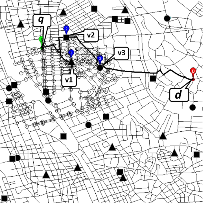
Fig. 1
An example of the safe-region for TRPQ.
In this paper, we propose the safe-region generation methods for CTRPQ. Figure
1 shows an example of the generated safe-region. In this example, before reaching the final destination
d, three data points
${v_{1}}$,
${v_{2}}$,
${v_{3}}$, selected from each category, are specified to visit. The bold line shows the optimal trip route, and the unfilled circle marked area is the generated safe-region. Even if a user veers from the optimal route, the route is still optimal if the current position is in the safe-region. Therefore, the user will only need to target the first visiting point (
${v_{1}}$) on the route if the user is still in the safe-region. By applying generated safe-regions to CTRPQ, the user does not need to send a new query while the user stays inside the safe-region. Therefore, using safe-region reduces the number of queries when the user veers from the query route. To the best of our knowledge, the safe-region generation method for TRPQ was first proposed in Ohsawa
et al. (
2016). This paper is the extended version of it.
The main contributions of this paper are as follows:
-
• three algorithms for safe-region generation in TRPQ are presented, and they are evaluated through intensive experiments;
-
• a new OSR query algorithm that is insensitive to the densities of data point sets is proposed;
-
• an on-the-fly road network distance materialization method is introduced for the efficient trip route path lengths comparison.
The rest of the paper is organized as follows. Related work is described in Section
2. In Section
3, snap-shot query methods for TRPQ are expressed. In Section
4, the first safe-region (SR) in CTRPQ is defined, and a naive algorithm for the safe-region is described. Two types of safe-region generation methods for CTRPQ are proposed in Section
5. Experimental evaluations are shown in Section
6. Finally, this paper is concluded in Section
7.
2 Related Work
In this section, we present related works for three topics: variation of trip route planning queries (TRPQ) queries, continuous queries, and the safe-region generation.
In existing works, several types of TRPQ algorithms have been proposed actively. A trip planning querying (TPQ) was first proposed in Li
et al. (
2005). In their method, a TPQ finds the shortest route from the starting point to the destination by visiting each data point from specified data categories sets sequentially. The visiting order is not specified in this query, and the minimum distance query (MDQ) algorithm, which gives the optimal route adaptable to road network distance, was proposed. Due to the lack of any restriction on the visiting order to data points categories, it requires processing time in proportion to
$M!{\Pi _{i=1}^{M}}N({C_{i}})$ where
M is the number of data point sets to be visited during the trip and
$N({C_{i}})$ is the number of data points in category
${C_{i}}$. Therefore, TPQ is practical when
M is small.
A similar approach called optimal sequenced route (OSR) queries was proposed by Sharifzadeh
et al. (
2005). In OSR queries, the visiting order is uniquely specified, and the processing time for OSR becomes obviously shorter than for the TPQ queries. Alternatively, in Chen
et al. (
2008), they proposed a multi-rule partial sequenced route (MRPSR) query. In their query, the visiting order of data point categories is specified by a set of rules, and the computational complexity lies between TPQ and OSR queries.
These types of queries require long processing time, and therefore, a precomputation method was proposed by Sharifzadeh and Shahabi (
2008) to shorten the processing time. Their method based on an extension version of the Voronoi diagrams is called the additively weighted Voronoi diagram (AWVD). However, this method can be adaptable only to a restricted version of a trip route planning query in which the final destination is not specified, and the trip route is terminated at the data point belonging to the last visiting category. For this reason, this method cannot be applied to our CTRPQ. Another problem is that the visiting categories order must be determined when AWVD is constructed.
If the trip route can be optimized by the total travelling time, it is more convenient for the user. Costa
et al. (
2015) proposed a method to optimize the route by the total travelling time, and they also considered changes of traffic conditions. They supposed a condition that the travelling time over an edge was time-dependent in OSR search.
In addition to snap-shot queries, continuous queries for moving objects have been actively researched since the year 2000. They can be classified into three main categories based on (1) query types, (2) Euclidean distance or road network distance, and (3) mobility of queries and data objects.
In the literature, varieties of continuous queries have been researched, consisting of range queries (Gedik and Liu,
2004; Prabhakar
et al.,
2002),
kNN query (Mouratidis
et al.,
2006), reverse NN (RNN) queries (Bentis
et al.,
2006; Xia and Zhang,
2006), spatial semi-join queries (Iwerks
et al.,
2004), path NN query (Chen
et al.,
2009), and skyline query (Huang
et al.,
2012).
In continuous queries, researches have been mainly focused on Euclidean distance in the pioneer studies. However, the movement of cars and humans are constrained on a road network in practical scenarios. To the best of our knowledge, a continuous query method in the road network distance was first proposed in Mouratidis
et al. (
2006). In their approach,
kNN objects are continuously monitored on road networks, where the distance between a query and a data object is determined by the length of the shortest path connecting them.
Continuous queries are generally realized based on the client-server model, and the task of a server is to continuously compute and update the result of each query according to the location changes of the moving objects. Consequently, queries are repeated periodically or with a certain distance move. However, when the frequency of updates becomes high, the load on the server becomes high.
To overcome overloads at the server side, the safe-region method was proposed in Prabhakar
et al. (
2002). When a moving object issues a
kNN or range query, the server generates a safe-region in which the query result remains unchanged. By the time the moving object leaves the safe-region, a new query result and the safe-region are requested to the server.
Alternatively, an efficient and effective monitoring technique based on the concept of a safe-region for range queries in road network distances was introduced in Cheema
et al. (
2011). They also proposed safe-region generation method for continuous R
kNN queries. Although safe-region generation methods have been actively researched, these algorithms were targeted to essentially simple query types.
For TRPQ, Nutanong
et al. proposed continuous detour query (CDQ) method, the simplest type of TRPQ (Nutanong
et al.,
2012). However, their method can only be applicable when the number of visiting data point categories is one. Additionally, their continuous query aimed for the fast re-calculation of new query result, and their interest was not the generation of the safe-region.
To the best of our knowledge, the first attempt of continuous trip route planning queries was introduced in Ohsawa
et al. (
2016) which was our previous work for CTRPQ with the objective to solve complex TRPQ queries. This paper is an extended version of the previous work. In the OSR query, the processing time in Htoo
et al. (
2012) method varies drastically depending on the visiting order of the data point categories. This paper proposes an algorithm insensitive to the distribution of data density. Moreover, this paper also proposes an on-the-fly network distance materialization method which is suitable for the safe-region generation.
3 Snap-Shot Query Methods for TRPQ
This section describes four types of snap-shot TRPQ algorithms. First, Section
3.1 defines TRPQ and introduces an existing method applicable in road network distances. Section
3.2 describes a fast TRPQ algorithm based on a best first search. This algorithm is improved in the average processing time. However, when the distribution densities of data object categories are substantially different from each other, the processing time is strongly affected by the search order of categories. Section
3.3 proposes an algorithm to ease the effect. The efficient safe-region generation algorithm proposed in Section
5.2 uses the TRPQ in Euclidean distance. Therefore, Section
3.4 introduces a Euclidean distance based TRPQ algorithm.
3.1 TRPQ and PNE Algorithm
Let ${C_{i}}$ be a category of the data points to be visited, and S be a sequence of ${C_{i}}$ to specify the visiting order. That is, $S=[{C_{1}},{C_{2}},\dots ,{C_{M}}]$, and here M is the length of S ($M=|S|$). This type of TRPQ is called the optimal sequenced route (OSR) query. A TRPQ finds the optimal trip route that gives the minimum trip cost. The cost is measured by various criteria, for example, the total length of the trip route, the total travelling time, and the total toll fees. In the rest of the paper, the cost is measured by the total length of the trip route, however, another cost can directly be applicable.
Definition 1 (Trip route planning query).
Given M categories of data point sets ${C_{i}}$ $(1\leqslant i\leqslant M)$, a current position q, and a final destination d, the trip route planning query (TRPQ) answers the minimum cost route while visiting each data point ${p_{i}}$ selected from ${C_{i}}$ $({p_{i}}\in {C_{i}})$ during the trip from q to d. The trip route is denoted by ${R_{1..M}}(q,d)$. The subscript $[1..M]$ shows each data point to visit in order from category one to category M. The trip route visiting from the first category is denoted by ${R_{M}}(q)$ for simplicity.
To simplify the explanation of the algorithm, we sometimes assume that the data point is on a road-network node. However, this restriction can be easily relaxed (Papadias
et al.,
2003).
Li
et al. (
2005) proposed MDQ algorithm for the trip route query in the road network distance in which the visiting order is not specified. Sharifzadeh
et al. (
2005) proposed the similar algorithm for OSR query called progressive neighbour exploration (PNE). Both algorithms gradually expand the search area by a similar way in Dijkstra’s shortest path algorithm. When a data point from the first visiting category
${C_{1}}$ is found, the algorithm starts a search targeting to a data point from the second visiting category (
${C_{2}}$). In parallel, the search is continued for the next nearest data point in the first category. Generally, when a data point belonging to the data set
${C_{k}}$ is found, the algorithm advances searching for a data point in
${C_{k+1}}$, and also continues the search for the next nearest data point in
${C_{k}}$. Repeating this process, the search is terminated when
M types of data points are found and the final destination point
d is reached.
Table
1 summarizes notations which frequently appear in the rest of the paper.
| Notation |
Meaning |
|
M |
Number of categories to be visited |
|
${C_{i}}$ |
Visiting data point set ($i\leqslant \imath \leqslant M$) |
|
q |
Current position of the moving object |
|
d |
Final destination of the trip |
|
${d_{E}}(x,y)$ |
Euclidean distance between x and y
|
|
${d_{N}}(x,y)$ |
Network distance between x and y
|
|
${R_{M}}(q)$ |
Optimal sequenced route starting at q, visiting M kinds of data, |
| |
then terminated at the final destination d
|
|
${L_{M}}(q)$ |
Total trip route length of ${R_{M}}(q)$
|
|
${R_{M}^{E}}(q)$ |
Optimal sequenced route searched in Euclidean distance |
|
${L_{M}^{E}}(q)$ |
Total trip route length of ${R_{M}^{E}}(q)$
|
|
${R_{2..M}}(p,d)$ |
Partial OSR starting from p, visiting each data point |
| |
from ${C_{2}}$ to ${C_{M}}$ in order, and then terminated at d
|
|
${L_{2..M}}(p,d)$ |
The total length of ${R_{2..M}}(p,d)$
|
3.2 TRPQ Applied A* Algorithm
The PNE algorithm needs long processing time, because the explored area in the road network expands circular for all-directions from
q. To shorten the processing time, Htoo
et al. (
2012) proposed a new TRPQ method based on A* algorithm. Hereafter, we call this algorithm OSRA.
Figure
2 shows the outline of OSRA. In this example, the search starts from
q, and then finds
${P_{1}^{1}}$ belonging to
${C_{1}}$. From this data point, a new search targeting to a data point in
${C_{2}}$ starts. In parallel, the search started at
q finds another data point in
${C_{1}}$ in the same way with PNE. A search path starting at
q, visiting
${P_{1}^{1}}$ and
${P_{1}^{2}}$ eventually reaches a node
${n_{a}}$ in Fig.
2. We call this route a partial route and denote it as
${\mathit{PR}_{1..2}}(q,{n_{a}})$. Generally, a partial route starting from a point
p, visiting
i types of data points, and reaching a node
n is shown as
${\mathit{PR}_{1..i}}(p,n)$, and the length as
${\mathit{LPR}_{1..i}}(p,n)$.
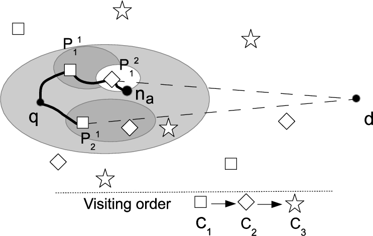
Fig. 2
Outline of trip route search by OSRA.
When a search reaches a network node
${n_{a}}$, all network nodes adjacent to
${n_{a}}$ are obtained by referring to the adjacency list, and the following record is composed for each adjacent node (
n). The records are then inserted into a heap H.
Here,
${C_{i}}$ is the next visiting data category,
L is the partial route length,
${\mathit{LPR}_{1..i}}(q,n)$.
$\mathit{Cost}$ is
$L+{d_{E}}(n,d)$, and the heap is ordered by
$\mathit{Cost}$ value.
${P_{\mathit{prev}}}$ is the last-visited data point that belongs to
${C_{i-1}}$. The reason of keeping already expanded node
${n_{a}}$ is to restore the trip route path by backtracking from
n to
q.
Repeating a deleteMin operation on H and the node expansion, the search area is gradually enlarged. The search is terminated when n in the record extracted from H is d (reaching the destination). Similarly in the Dijkstra’s algorithm and A* algorithm, once de-heaped, a record is registered in a closed set (CS). Every time a node is de-heaped from H, the node is checked whether it has already been included in CS, and the node is expanded only when it has not been included in CS to avoid the duplicated node expansion. In practice, CS is implemented by a hash table or a balanced binary tree. The difference of records in CS and H in a shortest path search is that the record in CS is assigned keys by a combination of the current node (n) and the previously visited data point ${P_{\mathit{prev}}}$, because a node in the road network is referred multiple times when the previously visited data point is different. For example, the search paths targeting to ${C_{1}}$ started from q to find the data points ${P_{1}^{1}}$ and ${P_{1}^{2}}$ which belong to ${C_{1}}$, and then new searches targeting to ${C_{2}}$ start from both of them. These two searches are executed independently. Therefore, a node that has been expanded by another search can be expanded again.
3.3 Sparse Category First Algorithm
The algorithm described in Section
3.2 runs fast when the distribution density of the data points are similar among categories. Contrary, when they differ greatly, the processing time is strongly affected by the visiting order of the data point categories.
This problem has been pointed out by Ohsawa
et al. (
2012). When the distribution densities of data points differ largely, the data point in the sparsest category must be determined first to shorten the processing time. Ohsawa
et al. (
2012) assumed that the densities of the data point sets were known in advance. However, this assumption does not always stand in real world applications. Therefore, this section proposes a method to investigate the distribution density of the data points set during the TRPQ.
Figure
3 shows the flow of the proposed method. In this example, the query (starting) point of the trip route search is
q, the final destination of the trip is
d. During the trip from
q to
d, visiting three kinds of data points are □, ♢, ⋆, in this order.
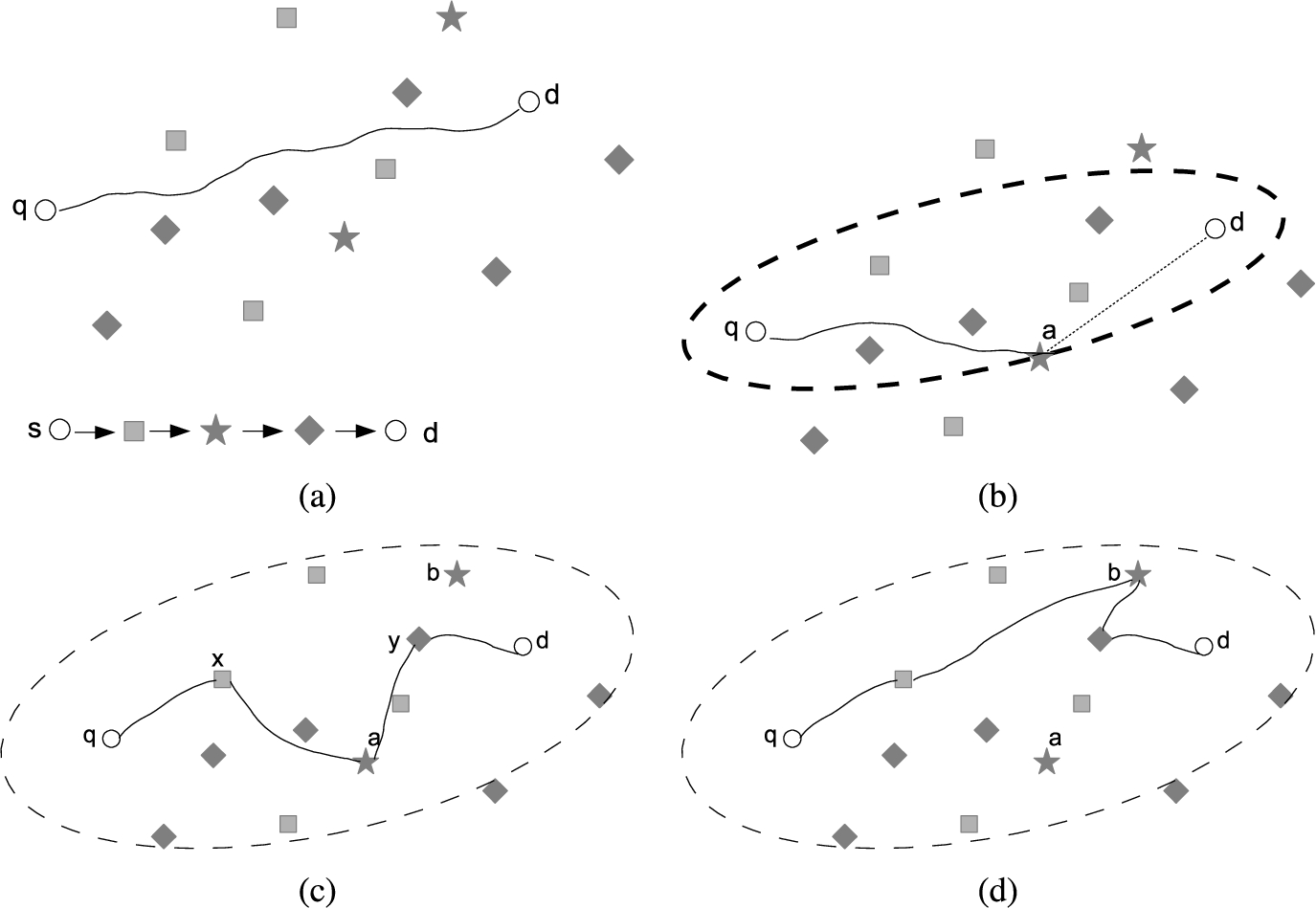
Fig. 3
Flow of sparse category first trip route search.
This query is performed by the following steps.
Search the shortest path connecting
q and
d by A* algorithm (Fig.
3(a)). This step only finds the shortest path. After the shortest path has been found, the contents of the heap (H) and the closed set (CS) are kept for the succedent steps.
Continue the node expansion by A* algorithm to find data points in each category (Fig.
3(b)). The expanded area grows larger, bounded by an ellipse whose focal points are
q and
d. Every time a data point is found in the procedure, the category of the found data point is marked as visited. Continue the above process until all categories are marked (at least one data point is found for all categories). Then, determine the last marked category
${C_{l}}$. Here,
${C_{l}}$ can be considered the most sparsely distributed category around the shortest path connecting
q and
d. In Fig.
3(b),
${C_{l}}$ is ⋆, and the first found data point in
${C_{l}}$ is
a.
The problem to find the trip route is divided into two sub-problems; one is to find the partial route from
q to
a via
$l-1$ data points selected each in
${C_{i}}$ $(1\leqslant i\leqslant l-1)$, and the other one is the route from
a to
d via
$M-l$ data points selected each in
${C_{j}}$ $(l+1\leqslant j\leqslant M)$. Then, merge two partial trip routes. As the result, the route
$q\to x\to a\to y\to d$ is found (Fig.
3(c)). Let the total length of the path be
T, and the length be
L. Notice that the route
T is still not guaranteed as the shortest trip route currently.
Resume the node expansion described in Step 2, and continue it while the following condition holds.
During the node expansion, add the found data points belonging to
${C_{l}}$ into a candidate data point set
$\mathit{Cand}$.
Search each trip route whose
l-th visiting point is the element in
$\mathit{Cand}$, in the same manner as described in Step 3. Then, answer the shortest route among them as the result. In Fig.
3(d), data point
b is found in the node expansion, and it is added into
$\mathit{Cand}$. Then, the partial route from
q to
b, and
b to
d is searched, and the total length is compared with
T. The shortest one is answered as the result.
Lemma 1.
The shortest trip route visits one of the data points in $\mathit{Cand}$ as the l-th visiting data point.
Proof.
Proof by contradiction. Suppose that the shortest route path visits a data point
p (
$\notin \mathit{Cand}$) as
l-th data point. The total length of the partial route starting from
q to
p and the partial route starting from
p to
d must be shorter than the first found trip route in Step 3, therefore the following equation stands.
${L_{1..l-1}}(q,p)\geqslant {d_{N}}(q,p)$ and
${L_{l+1..M}}(p,d)\geqslant {d_{N}}(p,d)$ stand, therefore,
However,
${d_{N}}(q,p)+{d_{E}}(p,d)>L$, because of the assumption that
p is not included in
$\mathit{Cand}$. Therefore,
This contradicts the assumption. □
3.4 Euclidean Distance Based TRPQ
TRPQ in Euclidean distance is considerably faster than in the road network distance. The length of the trip route obtained in Euclidean distance gives the lower bound of it in the road network distance. Ohsawa
et al. (
2012) proposed an efficient algorithm for TRPQ in Euclidean distance. R-tree is used as the spatial index to manage data points. The search descends the R-tree downward by referring to the minimum bounding rectangles (MBRs) in R-tree and creating routes. The search process is controlled by a heap, and the optimal route is found when the heap becomes empty. This algorithm can find the trip route in two or three orders of magnitude faster than the queries in road network distance. Therefore, the trip route searched in Euclidean distance can be used for pruning the search space in a road network.
4 Continuous Trip Route Planning Queries
In this section, the basic strategy of the safe-region (SR) in CTRPQ is presented in Section
4.1, and then a naive algorithm to obtain the safe-region is proposed in Section
4.2.
4.1 Safe-Region for CTRPQ
On the continuous trip route planning query (CTRPQ), the current position of a moving object (MO) changes continually. Fig.
4 shows the outline of a
safe-region (SR) in a CTRPQ. When a moving object at
q issues a query, the server searches the optimal trip route (TR) and generates the SR, and then sends them to the moving object. In this example, the optimal TR is the route visiting data points
${p_{1}}$ and
${p_{2}}$ in order (
$M=2$), selected each from
${C_{1}}$ and
${C_{2}}$ respectively. The MO always checks whether it remains inside of the SR, and when it leaves the SR, it requests a new optimal TR and the corresponding SR. On the other hand, when the MO follows the route and reaches
${p_{1}}$, belonging to the first visiting data category on the optimal route, the MO issues a new query starting from
${p_{1}}$ and the visiting category number is reduced to
$M-1$ (from
${C_{2}}$ to
${C_{M}}$), and then obtains a new SR. The procedure is repeated until the MO reaches the final visiting category (
${C_{M}}$). After passing through the data point in the final category, SR generation is not necessary anymore, because the problem is reduced to the shortest path search between the current position and the destination, and the whole road network can be considered as an SR.
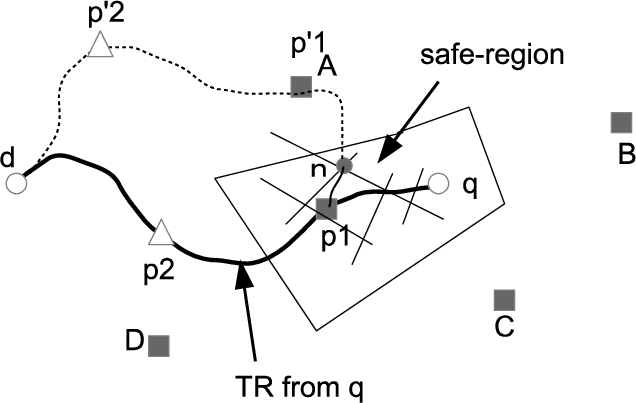
Fig. 4
Safe region in CTRPQ.
Definition 2 (Safe-region: SR).
An SR is the collection of the road link segments on which TRP queries issued at any point in the region give the same result. In other words, in the safe-region, ${R_{M}}(q)={R_{M}}({q^{\prime }})$, where q is the initial query point and ${q^{\prime }}$ is any position in the SR.
Therefore, while the MO remains in the SR, no new query is necessary even if MO veers from the first queried trip route. The SR of the trip route (TR) satisfies the following properties.
Property 1.
Let the first visiting data point on the TR searched from a point q be ${p_{1}}$ $(\in {C_{1}})$. The first visiting data point searched from any other point $({q^{\prime }})$ in the SR is identical with ${p_{1}}$.
Proof.
The proof is by contradiction. If the first visiting point of the query from ${q^{\prime }}$ is ${p^{\prime }_{1}}$ $(\ne {p_{1}})$, the TR queried from ${q^{\prime }}$ becomes ${R_{M}}({q^{\prime }})$ $(\ne {R_{M}}(q))$. This result contradicts the definition of the SR. Therefore, this property holds. □
Property 2.
When a TR is given, the rest of the route after visiting the data point in the first category $({C_{1}})$ is uniquely determined except for the case of plural TRs which give the same length.
Proof.
The queried TR is the optimal (the shortest) route. Therefore, if the first visiting data point (${p_{1}}$) is given, the rest of the TR is uniquely determined. □
Therefore, to find the safe-region, it is enough to search the area on the road network where the first visiting data point for the TRs is the same.
By Property
1, the first visiting data point is the same if TR is queried in the SR. Contrary, the first visiting data points are different on the TRs queried by two end points (network nodes) of a network link across the SR border. In this case, the shortest TR queried from a node included in the SR goes through
${p_{1}}$ (
$\in {C_{1}}$), and the shortest TR queried from the other node of the link goes through the other data point
${p^{\prime }}$ (
$\in {C_{1}}$). Hereafter,
${p^{\prime }}$ is called a
rival object (RO). For example, in Fig.
4, data objects A, B, C, and D are rival objects against
${p_{1}}$.
Definition 3 (Minimal rival object set).
Minimal rival object set is the set of necessary and sufficient rival objects to form an SR.
4.2 Basic Algorithm for Safe-Region Generation
This section describes a naive algorithm to generate an SR.
Figure
5 shows the basis for the safe-region generation. In the figure,
q is the current position of an MO,
d is the final destination, the thick line shows
${R_{2}}(q)$ where two kinds of data points are visited from
q before reaching
d. By Property
2, the TR queried by a point in the SR always passes through
${p_{1}}$ as the first visiting point.
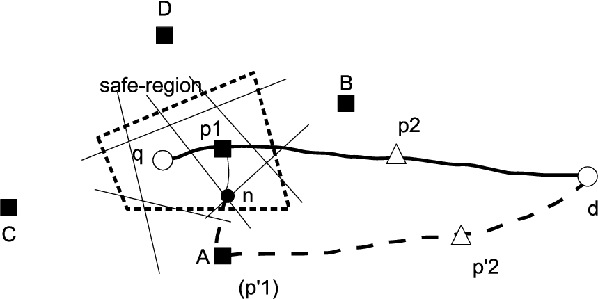
Fig. 5
Rival data object.
The SR to be generated is a region where the first visiting point on the TR is ${p_{1}}$. Therefore, the SR can be obtained by expanding the area starting from ${p_{1}}$ and checking whether the first visiting point on the queried TR is ${p_{1}}$ or not at each expanding node. This area expansion is performed in the similar manner in the Dijkstra’s shortest path algorithm, controlled by a minimum heap managing the records with the format $\langle \mathit{cst},n,\ell \rangle $. Here, n is the current noticed node in the road network, $\mathit{cst}$ is ${d_{N}}({p_{1}},n)$, and ℓ is a road segment where one edge is n and the other edge is already visited node by the node expansion. The heap is sorted in ascending order by $cst$ value. And the record, once obtained by the heap, is added to the closed set (CS) to avoid duplicated checks.
When the de-heaped record from the heap is
r, the TR starting from
$r.n$ (
${R_{M}}(r.n)$) is searched by the algorithm presented in Section
3.2 or
3.3. If the first visiting data point in the TR is
${p_{1}}$, the link
$r.\ell $ is added into the SR. Then, the adjacent links to
$r.n$ are obtained by the adjacency list, and the following procedure is done for each link. Let the link be
${\ell _{p}}$, and the opposite end point of
$r.n$ be
${n_{p}}$. If
${\ell _{p}}$ has not been registered in CS, a new record
$\langle n.cst+|{\ell _{p}}|,{n_{p}},{\ell _{p}}\rangle $ is composed, and added into the heap. The above sequence of steps is called the
node expansion. On the other hand, when the first visiting data point in the TR does not meet
${p_{1}}$, the node is not further expanded because the node is not included in the SR. However, even in this case, a part of the link (
$r.\ell $) can be included in the SR. Therefore, if the query condition for a part of the link is satisfied, the part will be added into the safe-region.
Generally, the SR is not given as a closed region in the similar way in the region formed by Voronoi decomposition. For example, when data points in ${C_{1}}$ are distributed only around the centre of the road network, the TR will contain the same point as the first visiting data point even if the query point is located far away. In such case, the SR becomes large, and the processing time becomes very long, because the processing time is proportional to the number of nodes contained in the SR. We can assume the moving objects do not veer far away from the TR route. Therefore, in practical way, we set an upper limit of the node number contained in the SR, and when the number is exceeded, we terminate the expansion of the SR, and send the result SR to the moving object.
5 Safe-Region Generation Method for CTRPQ
This section proposes two efficient algorithms for safe-region generation. The first one is the preceding rival addition algorithm, and the second one is the tardy rival addition algorithm.
5.1 Fundamental Strategy for Proposed Methods
If the minimal rival object set (MROS) is given in advance, the safe-region can be obtained easily. In this case, the TR starting from each object r ($\in RO$), ${R_{2..M}}(r,d)$ can be searched in advance. So, we also obtain ${L_{2..M}}(r,d)$ in advance.
Figure
6 shows an example of this assumption. The first visiting data object of the queried TR is
p where (
$p\in {C_{1}}$), and the SR is created around it.
${d_{p}}$ shows the length of the trip route starting from
p (
${L_{2..M}}(p,d)$). Five data points from
${r_{1}}$ to
${r_{5}}$ are the rival objects of
p. As mentioned above, the length of the TR starting from each data object can be calculated in advance. The SR can be created fast in this preparation.
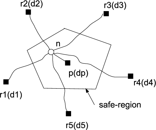
Fig. 6
Minimal rival objects set.
As described in Section
4.2, the search area is gradually enlarged while the TR starting from a network node
n visits
p as the first visiting point. This check can be done by comparing the TR length starting from
n and the first visiting point
p with other rival object as the first visiting point, using precomputed
${d_{i}}$.
n is included in the SR while the next inequality stands.
This method can avoid repetition of the time consuming TR queries, therefore, a fast SR generation can be expected.
The main issue to consider is how to obtain minimal rival object set in advance. In the rest of this section, two algorithms are presented to settle this problem.
5.2 Preceding Rival Addition Algorithm
We need to find enough ROs to affect the shape of the safe-region rapidly. When a TR is searched in Euclidean distance, we can obtain the candidate of RO fast. The length of TR in Euclidean distance gives the lower bound of TR searched in road network distance, i.e. ${L_{M}}(q)\geqslant {L_{M}^{E}}(q)$. Between the length of the TR starting ${p_{1}}$ $(\in {C_{1}})$ and a length of another TR starting from ${p^{\prime }_{1}}$ $(\in {C_{1}})$, the following property stands.
Property 3.
Let ${p_{1}}$ be the first visiting point in a TR. When a network node n is included in the safe-region of the TR, a data point ${p^{\prime }_{1}}$ $(\in {C_{1}})$ can be an RO if the following inequality is satisfied.
Here, the sub-script $2..M$ shows a route starting from the second category to the M-th category.
Proof.
If the length of a TR passing through
${p^{\prime }_{1}}$ is shorter than the TR passing through
${p_{1}}$, the following inequality stands.
By triangle inequality,
Then,
Therefore, the given inequality stands. □
The procedure described in Section
4.2 enlarges the search area gradually while the first visiting data point is
${p_{1}}$. To perform this, the time consuming TR query in road network distance must be repeated at every node. Therefore, we contrive a method to shorten the processing time to form an SR by reducing the number of the rival objects. By enlarging the SR, all possible rival objects that satisfy Property
3 are searched. For each rival object (
${p^{\prime }_{1}}\in {C_{1}}$), the length of the TR (i.e.
${L_{2..M}}({p^{\prime }_{1}},d)$) is obtained in advance. Under this preparation, the shortest TR route starting from an expanding node
n can be obtained only by the shortest path search between
n and each rival object.
Algorithm 2
AddCandidate.
Algorithm 3
minDistInSet.
Algorithm
1 shows the pseudocode of the algorithm described above. The parameter
q is the current position of the MO,
d is the final destination of the trip, and
M is the number of categories to be visited. Besides these parameters, the procedure refers to R-tree indexes managing each data point set (
${C_{i}}$). They are referred to
$\mathit{RTree}[i]$ $(1\leqslant i\leqslant M$). The lines from 2 to 4 initialize the heap H, the closed set CS, the result set of segments to be included in the SR, and the set of the candidate rival objects RO.
The function initialize performs the following initialization steps.
While H is not empty, lines from 6 to 21 are repeated. At line 7, a record having minimum d value is de-heaped from H, and the record is registered into CS at line 8.
In line 9,
addCandidate searches TR in Euclidean distance from
$r.n$ while Eq. (
6) is satisfied, and then the first visiting object in the searched Euclidean TR is added into the rival object set RO. In this search,
${p_{1}}$ and found rival candidate objects are successively removed from set
${C_{1}}$ (this means that the found rival objects are removed from RTree[1]).
Line 10 calculates the distance from the current node $r.n$ to each rival object and determines the minimum distance among them. If the distance is smaller than $r.d$, it means a route visiting the rival object is shorter than the route visiting ${p_{1}}$, in other words, $r.n$ is not included in the SR. In this case, $r.\ell $ is divided into two segments, and the part TR passing through ${p_{1}}$ which is shorter than the rival object is added into SR (line 12). On the other hand, if the route visiting ${p_{1}}$ is shorter, the whole $r.\ell $ is added into SR (line 14).
In line 16, all links neighbouring to $r.n$ are obtained by referring to the adjacency list. Then new records are composed, and they are inserted into H.
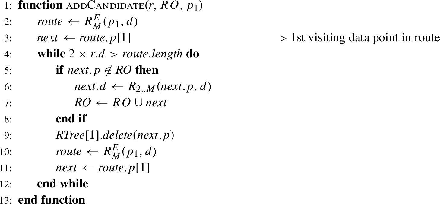
Algorithm
2 shows
AddCandidate, which obtains RO set incrementally. New objects, which satisfy Eq. (
6), are obtained and added into RO. TR in Euclidean distance, starting from
${p_{1}}$ and visiting
M data points, is searched incrementally in line 2, and the first visiting data point (
$\in {C_{1}}$) is assigned to the variable
$\mathit{next}$. From line 4, a new rival object (
$\mathit{next}$) is searched, and while it satisfies Property
3, it is added into RO.
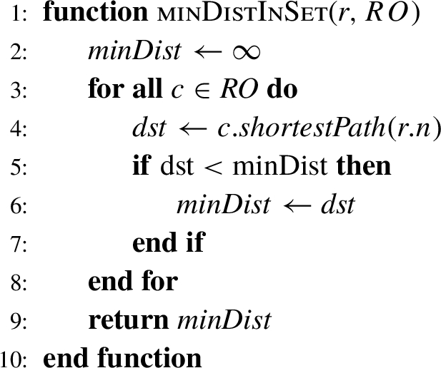
Algorithm
3 finds the shortest TR route to reach
$r.n$ among the rival objects. Each RO (
c) preserves the TR distance from the position to
d. Therefore, the total TR distance from a node
n can be easily calculated by adding
${d_{N}}(n,c)$ to the preserved length
${L_{2..M}}(c,d)$.
5.3 Verification in Road Network Distance
In Algorithm
3, the road network distance between an expanding node (
$r.n$) and a rival object is calculated repeatedly, while the safe-region gradually enlarges (
$r.n$ is changed). For this calculation, the existing pair-wise A* algorithm can be applied. Though, A* algorithm is efficient enough to search the shortest path in the road network, the distance queries are repeated multiple times. Therefore, we contrive a method for the distance calculation to shorten the processing time. This is a type of on-the-fly network distance materialization method.
Before presenting our method, we examine a conventional pair-wise A* algorithm. When two points s and e on a road network are given, the road network distance ${d_{N}}(s,e)$ between these two points are calculated by the A* algorithm as following. In the algorithm, a heap (H) is used to retrieve the minimum cost record, and the record format in H is $\langle c,n,d\rangle $ where c is the cost (${d_{N}}(s,n)+{d_{E}}(n,e)$), n is a current noticed road network node, and d is the road network distance from s to the current node n (i.e. ${d_{N}}(s,n)$). To prevent duplicated processing, once de-heaped, a node is registered in a closed set (CS).
The heap (H) is initialized by the record $\langle {d_{E}}(s,e),s,0\rangle $, then the repetition of the following steps starts.
De-heap a record (r) having the minimum c value from H.
If $r.n$ is already in CS, go to Step 1, else insert r into CS.
If $r.n=e$, the path to e has been found, then return $r.d$ value as the shortest path length.
Obtain adjacent nodes to $r.n$ referring to the adjacency list. For each adjacent node n, compose $\langle {d_{N}}(r.n,n)+r.d+{d_{E}}(n,e),n,{d_{N}}(r.n,n)+r.d\rangle $, then insert it into H.
Lemma 2.
Let s be a start point, $r.n$ be a current node and $r.d$ be a distance from s to $r.n$. If a record r is included in a closed set $CS$, then $r.d$ is the shortest distance from s to $r.n$.
The proof of this lemma is shown in Htoo
et al. (
2013).
In Algorithm
3, the road network distance from
$r.n$ to a candidate object
o is calculated. To obtain the distance, the pair-wise A* algorithm can be applied. Figure
7(a) shows an example of how to apply it. Here, □ shows the nodes in H, and × shows the nodes in CS.

Fig. 7
The efficiency in road network distance calculation.
The positions of ROs (in this example
s) are fixed, on the other hand,
$r.n$ moves around the surrounding area of
q. Figure
7(b) shows this situation. Nodes
${n_{1}}\sim {n_{4}}$ are the adjacent nodes of
q. Following
${d_{N}}(o,q)$ searching,
${d_{N}}(o,{n_{1}})\sim {d_{N}}(o,{n_{4}})$ are requested. In this situation, similar explorations on the network are repeated when we apply the pair-wise A* algorithm.
This repetition can be efficient by reusing the contents of H and CS. According to Lemma
2, the records in CS have
${d_{N}}(o,n)$ as
d value in the record. Therefore, if a destination node is already in CS,
${d_{N}}(o,n)$ can be obtained to refer
$r.d$.
When a destination is not in CS, proceed according to the following steps.
Recalculate
c value of the all records in H by
Here,
$r.n$ is the
n (node) in the record
r.
Resume the search procedure using recalculated H. Step(1) is executed only for the nodes in the heap and no disk IO is necessary, therefore, the CPU time of this step is short.
Figure
7(b) shows the status after the distance to
${n_{1}}$–
${n_{4}}$ have been obtained. As shown in this figure, the number of nodes in CS and in H are considerably smaller than five times of them in Fig.
7(a). The difference of the number of node expansion times is directly proportional to the processing time.
5.4 Tardy Rival Addition Algorithm
In the PRA algorithm, the number of rival objects (RO) increased rapidly. Every time a candidate RO (
o) is found by Euclidean distance search, the TR from
o visiting
$M-1$ categories must be determined in the road network distance. Therefore, the total processing time increases in proportion to the number of the ROs. In addition to determining the TR in the Euclidean distance, a found candidate RO must be removed from R-tree index to perform the incremental search in the CTRPQ algorithms (see line 8 in Algorithm
2). For this object deletion, R-tree index is needed to be copied into the main memory. When a R-tree index is referred, a least recently used (LRU) buffer is used to improve the IO response. Therefore, this deletion is performed inside the buffer region to avoid to soil R-tree. To solve these problems, we propose the following approximated algorithm called tardy rival addition (TRA) algorithm.
The principle of TRA is to find the candidate rival objects by nearest neighbour query targeting to ${C_{1}}$ object from the currently noticed node. The search area is gradually enlarged as the same with the basic algorithm and the PRA. During the enlargement of the SR area, the nearest neighbour object except ${p_{1}}$ in ${C_{1}}$ from the current noticed node is searched. And then, the object is added into the RO set. In this method, the RO search can be limited by the vicinity of the current node, therefore, the number of the ROs is apt to be reduced.
On the other hand, this method can overlook the RO which makes an actual shape of the SR. When enough ROs are not found, the size of the SR tends to be enlarged larger than the actual size. However, by the result of the experiment, this enlargement is smaller than a few percentage of the real SR size.
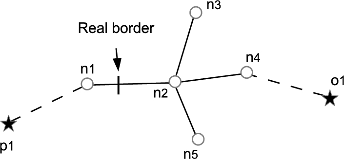
Fig. 8
Safe-region generation by TRA.
Figure
8 shows a situation for the SR generation. In this figure, when node
$n1$ and
$n2$ are checked, the route passing through
${p_{1}}$ is considered the shortest because the RO has not been found, and then the expansion is continued. When node
$n4$ is checked, the object
$o1$ is found as an RO by the NN search at
$n4$, and also it is found that the TR length passing through
$o1$ is shorter than the TR passing through
$p1$ at node
$n4$. In this case, apparently
$n4$ is not included in the SR. However,
$n2$ and
$n1$ also have a possibility that these nodes are not included in the SR, because
$o1$ has not been in the RO set when they are checked. Therefore, the check is needed to trace back along the path to reach
$n4$. In this case, when
$n2$ is tested again, it is found that
$n2$ is not included in the SR, and while testing on
$n1$, it is found that it is included in the SR. In this situation, the border of the SR is determined on the link between
$n1$ and
$n2$. A defect of this method is that TRA does not guarantee to find enough ROs to form an exact shape of the SR, because there can be a possibility of the existence of ROs which have not been found yet.
In comparison with PRA, TRA does not need to remove the rival objects from the R-tree, and thus the copy of the R-tree managing ${C_{1}}$ is not necessary.
The flow of the procedure for the TRA is the same with PRA. The only difference is in the function
addCandidate. This algorithm is presented in Algorithm
4. The function NN in line 2 returns the nearest neighbour in
${C_{1}}$ but except
${p_{1}}$.

Algorithm 4
AddCandidate for TRA.
6 Experimental Results
To evaluate the algorithms proposed in this paper, we conducted several experiments. The algorithms were implemented by Java. In these experiments, we used a real road map (167 km${^{2}}$) with road network nodes 16 284 and 24 914 links that cover an area of a city, and generated data points sets with various densities. For example, the density of 0.001 means that a data point exists at every 1 000 road edges. The size of the area is not so large, however, this type of query is apt to be used by a user for a trip route search in an unknown city, and hence the search area is restricted in a city.
Figure
9 shows results for the performance of the sparse category first OSR algorithm presented in Section
3.3 and the OSRA. Figure
9(a) shows the processing time to search TR visiting four kinds of data points, the density
${C_{1}}$ is 0.001 and the rest (
${C_{2}}\sim {C_{4}}$) are 0.02. The horizontal axis shows the route length in kilometer (km). Figure
9(a) shows the result in which the first visiting category is the sparsest. The sparse category first algorithm (SCFA) requires longer processing time than OSRA. This is because SCFA requires additional processing to determine the sparsest category.
In the rest of Fig.
9(b)–(d) the sparsest category shifts to the second (b), to the third (c), and to the last visited (d). According to the sparsest category visited later, the processing time of OSRA becomes longer. Contrary, SCFA turns to be relatively faster than OSRA.
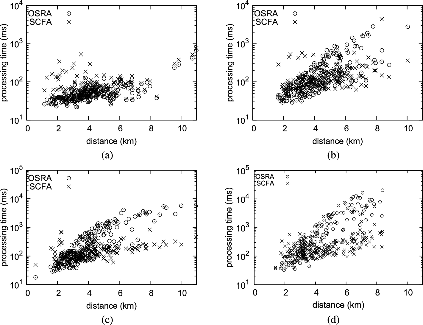
Fig. 9
Shift the sparsest category visiting order.
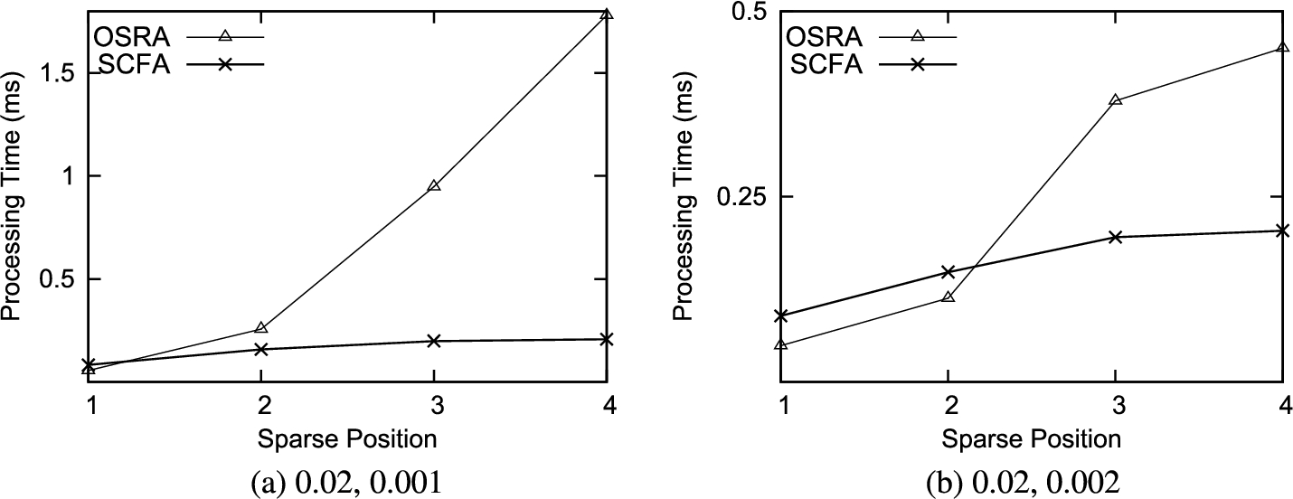
Fig. 10
Processing time vs. visiting order of the sparsest category.
Figure
10 shows the average processing time of TR search. Figure
10(a) shows the average processing time of the same experiment with Fig.
9, and Fig.
10(b) shows the result that the density of dense category is 0.02 and its sparse category is 0.002. As shown in this result, the processing time of OSRA increases according to the position of the sparsest category. On the other hand, the processing time of SCFA does not affect the visiting order of the sparsest category.
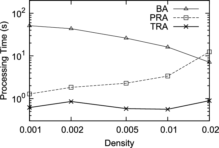
Fig. 11
Processing time for SR when $M=3$.
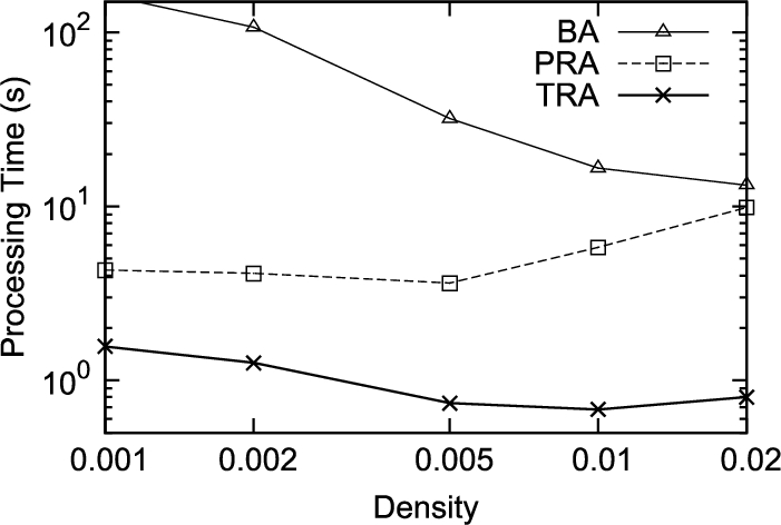
Fig. 12
Processing time for SR when $M=4$.
Figure
11 compares the processing time of the basic algorithm (BA), PRA, and TRA when
$M=3$. In the rest of experiment, OSRA is used for TR search, because the density of all data point sets is the same. The basic algorithm requires very long processing time especially when the density of the data points is low. This is because when the density is low, the size of the SR becomes larger, and according to the enlargement in size, the number of repetitions to find TR in the road network distance becomes large. The processing time becomes low in accordance with the density increase. Contrary, the processing time of PRA increases when the density becomes high. This is because the number of the candidate rival objects also increases when the density is high. Therefore, the execution times of line 6 in Algorithm
2 increase, and this is dominant in PRA processing. TRA shows stable and low processing time independent of the density distribution.
Figures
12 and
13 show the processing time when
$M=4$ and
$M=5$ respectively. According to the increase of
M, the processing time of all algorithms increases, however, PRA and TRA keep remaining lower in the processing time than BA.
In a trip, after a MO has reached the first visiting data point, a new SR targeting to the second visiting data point is generated. Figure
14 shows the processing time to generate the second SR in a trip. In this figure, only PRA and TRA are compared, because BA needs long processing time especially when the density of data points is low. The last number in the legend shows
M number. For example, PRA5 shows the result when
$M=5$, and the value shows the processing time to generate the SR for the TR visiting the rest four data points.
7 Conclusion
This paper firstly discussed trip route query (targeting to OSR) algorithms in the road network distances, and proposed an algorithm whose processing time is not sensitive to the distribution of the density of data point sets. The processing time of OSR query usually increases greatly when the distribution density of the last visiting data point set is sparse. To cope with this problem, we proposed the sparse category first algorithm. Through experimental evaluations, we demonstrated that the algorithm is insensitive to the distribution of the data density.
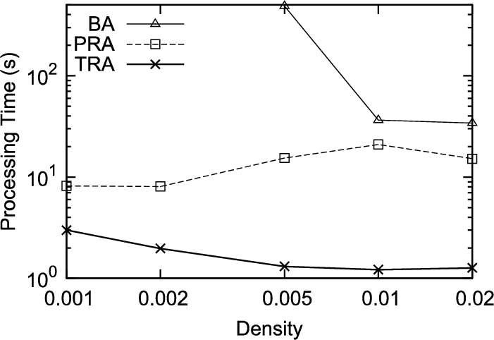
Fig. 13
Processing time for SR when $M=5$.
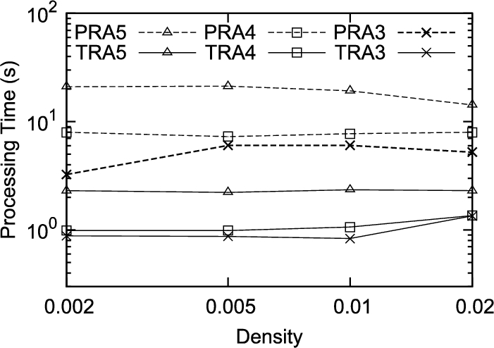
Fig. 14
Search safe region of next data point.
Moreover, this paper proposed three types of safe-region generation algorithms for continuous trip planning queries. The first one is the BA, it takes long processing time. The PRA searches the rival objects in Euclidean distance, and then it compares the length of the trip route between the target object and the rival objects. This algorithm outperforms the BA in processing time, however, it is apt to find many redundant rival objects when the density of the data point is high. This characteristic causes long processing time especially when the data point density of the first visiting data point category is high. The last proposed algorithm is the TRA. This algorithm finds lesser rival objects than the PRA, therefore the processing time is very short. However, the main issue of this algorithm is that it gives about 5% larger than PRA in the safe-region size. This is because the TRA is not guaranteed to find minimal rival objects. A countermeasure to this problem is future works.

