This section intends to exemplify the functionality and suitability of the propounded methodology for applications in a location selection issue for a construction company in complex uncertain circumstances. Moreover, this section puts into effect two comparative studies to scrutinize the helpfulness and merits of the current technique.
4.1 Realistic Application and Discussions
The multiple-criteria choice case investigated by Chen
et al. (
2021) focused on the issue of a construction company finding an appropriate location to put up a new apartment. In order to find the most suitable location, the construction company evaluates four location options (
${a_{1}}-{a_{4}}$) for constructing new apartments predicated on the four performance criteria. The performance criteria consist of land cost (
${c_{1}}$), surrounding environment (
${c_{2}}$), technological capability (
${c_{3}}$), and lease value (
${c_{4}}$). Fig.
3 provides a profile of the location selection issue under study.
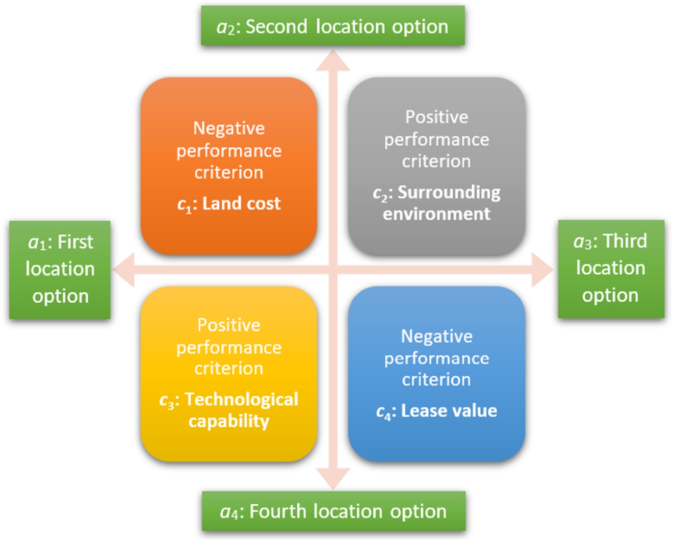
Fig. 3
Profile of the location selection issue of a construction company for building new apartments.
In Step 1, the two limited sets of choice options and performance criteria were designated as
$A=\{{a_{1}},{a_{2}},{a_{3}},{a_{4}}\}$ and
$C=\{{c_{1}},{c_{2}},{c_{3}},{c_{4}}\}$, respectively. Herein, the set
C was separated into two parts: one is the collection of positive criteria
${C_{\textit{Po}}}=\{{c_{2}},{c_{3}}\}$; the other is the collection of negative criteria
${C_{\textit{Ne}}}=\{{c_{1}},{c_{4}}\}$. In Step 2, in conformity with the expert’s professional opinions, the normalized (standardized) weights were given by
$({w_{1}},{w_{2}},{w_{3}},{w_{4}})=(0.2,0.1,0.3,0.4)$. In Step 3, the expert evaluated the location options one by one based on the four performance criteria, and the relevant evaluation data were expressed in terms of T-SF information, as revealed in Table
2. The data fields contain the T-SF performance rating
${t_{ij}}=({\mu _{ij}},{\eta _{ij}},{\nu _{ij}})$ and its associated refusal-membership
${\gamma _{ij}}$, where the positive-integer exponent
$q=3$ and
${\gamma _{ij}}=\sqrt[3]{1-{({\mu _{ij}})^{3}}-{({\eta _{ij}})^{3}}-{({\nu _{ij}})^{3}}}$. Taking
${t_{13}}=(0.81,0.62,0.11)$ as an illustration,
${\gamma _{13}}=\sqrt[3]{1-{0.81^{3}}-{0.62^{3}}-{0.11^{3}}}=0.61$. In Step 4, the T-SF characteristics were generated by
${T_{i}}=\{\langle {c_{j}},{t_{ij}}\rangle \hspace{0.1667em}|\hspace{0.1667em}{c_{j}}\in C\}=\{\langle {c_{j}},({\mu _{ij}},{\eta _{ij}},{\nu _{ij}})\rangle \hspace{0.1667em}|\hspace{0.1667em}{c_{j}}\in \{{c_{1}},{c_{2}},{c_{3}},{c_{4}}\}\}$ for each location option
${a_{i}}$. For example,
${T_{1}}=\{\langle {c_{1}},(0.43,0.20,0.61)\rangle ,\langle {c_{2}},(0.54,0.35,0.63)\rangle ,\langle {c_{3}},(0.81,0.62,0.11)\rangle ,\langle {c_{4}},(0.18,0.33,0.66)\rangle \}$.
Table 2
Data of the T-SF performance rating ${t_{ij}}$ (with the refusal-membership ${\gamma _{ij}}$) in the location selection problem.
| ${c_{j}}$ |
${t_{1j}}=({\mu _{1j}},{\eta _{1j}},{\nu _{1j}})$ |
${\gamma _{1j}}$ |
${t_{2j}}=({\mu _{2j}},{\eta _{2j}},{\nu _{2j}})$ |
${\gamma _{2j}}$ |
${t_{3j}}=({\mu _{3j}},{\eta _{3j}},{\nu _{3j}})$ |
${\gamma _{3j}}$ |
${t_{4j}}=({\mu _{4j}},{\eta _{4j}},{\nu _{4j}})$ |
${\gamma _{4j}}$ |
| ${c_{1}}$ |
$(0.43,0.20,0.61)$ |
0.88 |
$(0.14,0.32,0.74)$ |
0.82 |
$(0.75,0.12,0.41)$ |
0.80 |
$(0.35,0.44,0.83)$ |
0.67 |
| ${c_{2}}$ |
$(0.54,0.35,0.63)$ |
0.82 |
$(0.26,0.17,0.26)$ |
0.99 |
$(0.59,0.29,0.13)$ |
0.92 |
$(0.91,0.12,0.49)$ |
0.50 |
| ${c_{3}}$ |
$(0.81,0.62,0.11)$ |
0.61 |
$(0.77,0.23,0.55)$ |
0.71 |
$(0.56,0.22,0.36)$ |
0.92 |
$(0.63,0.11,0.27)$ |
0.90 |
| ${c_{4}}$ |
$(0.18,0.33,0.66)$ |
0.88 |
$(0.61,0.34,0.57)$ |
0.82 |
$(0.11,0.14,0.45)$ |
0.97 |
$(0.31,0.36,0.84)$ |
0.69 |
In Step 5, the T-SF weighted performance rating
${t_{ij}^{w}}$ was computed using Eq. (
3). To give an instance,
${t_{13}^{w}}=(n\cdot {w_{3}})\odot {t_{13}}=(4\times 0.3)\odot {t_{13}}=({[1-{(1-{0.81^{3}})^{1.2}}]^{1/3}},{[{(1-{0.81^{3}})^{1.2}}-{(1-{0.81^{3}}-{0.62^{3}})^{1.2}}]^{1/3}},{[{(1-{0.81^{3}}-{0.62^{3}})^{1.2}}-{(1-{0.81^{3}}-{0.62^{3}}-{0.11^{3}})^{1.2}}]^{1/3}})=(0.8422,0.6136,0.1060)$, where the refusal-membership
${\gamma _{13}^{w}}=\sqrt[3]{1-{0.8422^{3}}-{0.6136^{3}}-{0.1060^{3}}}=0.5544$. The computed outcomes of
${t_{ij}^{w}}$ and
${\gamma _{ij}^{w}}$ are revealed in the third and fourth columns of Table
3. Moreover, the T-SF weighted characteristics were determined by the use of
${T_{i}^{W}}=\{\langle {c_{j}},{t_{ij}^{w}}\rangle \hspace{0.1667em}|\hspace{0.1667em}{c_{j}}\in C\}=\{\langle {c_{j}},({\mu _{ij}^{w}},{\eta _{ij}^{w}},{\nu _{ij}^{w}})\rangle \hspace{0.1667em}|\hspace{0.1667em}{c_{j}}\in \{{c_{1}},{c_{2}},{c_{3}},{c_{4}}\}\}$ for each
${a_{i}}$. As an illustration,
${T_{1}^{W}}=\{\langle {c_{1}},(0.4003,0.1867,0.5750)\rangle ,\langle {c_{2}},(0.4046,0.2683,0.5031)\rangle ,\langle {c_{3}},(0.8422,0.6136,0.1060)\rangle ,\langle {c_{4}},(0.2104,0.3841,0.7406)\rangle \}$.
Table 3
Outcomes relevant to the T-SF weighted performance rating ${t_{ij}^{w}}$ and the refusal-membership ${\gamma _{ij}^{w}}$ ($q=3$).
| ${a_{i}}$ |
${c_{j}}$ |
${t_{ij}^{w}}=({\mu _{ij}^{w}},{\eta _{ij}^{w}},{\nu _{ij}^{w}})$ |
${\gamma _{ij}^{w}}$ |
${({\mu _{ij}^{w}})^{q}}$ |
${({\eta _{ij}^{w}})^{q}}$ |
${({\nu _{ij}^{w}})^{q}}$ |
${({\gamma _{ij}^{w}})^{q}}$ |
Squared sum∗
|
| ${a_{1}}$ |
${c_{1}}$ |
(0.4003, 0.1867, 0.5750) |
0.9042 |
0.0641 |
0.0065 |
0.1901 |
0.7393 |
0.5868 |
|
${c_{2}}$ |
(0.4046, 0.2683, 0.5031) |
0.9233 |
0.0662 |
0.0193 |
0.1274 |
0.7871 |
0.6405 |
|
${c_{3}}$ |
(0.8422, 0.6136, 0.1060) |
0.5544 |
0.5974 |
0.2310 |
0.0012 |
0.1704 |
0.4393 |
|
${c_{4}}$ |
(0.2104, 0.3841, 0.7406) |
0.8082 |
0.0093 |
0.0567 |
0.4062 |
0.5278 |
0.4469 |
| ${a_{2}}$ |
${c_{1}}$ |
(0.1300, 0.2974, 0.7002) |
0.8564 |
0.0022 |
0.0263 |
0.3433 |
0.6282 |
0.5132 |
|
${c_{2}}$ |
(0.1919, 0.1258, 0.1928) |
0.9946 |
0.0071 |
0.0020 |
0.0072 |
0.9838 |
0.9679 |
|
${c_{3}}$ |
(0.8036, 0.2345, 0.5538) |
0.6682 |
0.5189 |
0.0129 |
0.1699 |
0.2983 |
0.3873 |
|
${c_{4}}$ |
(0.6963, 0.3758, 0.6098) |
0.7259 |
0.3376 |
0.0531 |
0.2267 |
0.3826 |
0.3146 |
| ${a_{3}}$ |
${c_{1}}$ |
(0.7080, 0.1156, 0.3965) |
0.8345 |
0.3549 |
0.0015 |
0.0623 |
0.5812 |
0.4677 |
|
${c_{2}}$ |
(0.4446, 0.2244, 0.1009) |
0.9654 |
0.0879 |
0.0113 |
0.0010 |
0.8998 |
0.8175 |
|
${c_{3}}$ |
(0.5914, 0.2307, 0.3766) |
0.8994 |
0.2068 |
0.0123 |
0.0534 |
0.7275 |
0.5750 |
|
${c_{4}}$ |
(0.1286, 0.1637, 0.5210) |
0.9480 |
0.0021 |
0.0044 |
0.1414 |
0.8521 |
0.7461 |
| ${a_{4}}$ |
${c_{1}}$ |
(0.3254, 0.4109, 0.8012) |
0.7255 |
0.0344 |
0.0694 |
0.5143 |
0.3818 |
0.4163 |
|
${c_{2}}$ |
(0.7542, 0.1171, 0.5083) |
0.7595 |
0.4289 |
0.0016 |
0.1313 |
0.4381 |
0.3932 |
|
${c_{3}}$ |
(0.6634, 0.1147, 0.2812) |
0.8812 |
0.2920 |
0.0015 |
0.0222 |
0.6843 |
0.5540 |
|
${c_{4}}$ |
(0.3615, 0.4165, 0.8922) |
0.5544 |
0.0472 |
0.0722 |
0.7101 |
0.1704 |
0.5408 |
In Step 6, based on the universal and null T-SF sets, the T-SF characteristic
${T_{+}}=\{\langle {c_{1}},(0,0,1)\rangle ,\langle {c_{2}},(1,0,0)\rangle ,\langle {c_{3}},(1,0,0)\rangle ,\langle {c_{4}},(0,0,1)\rangle \}$ because of
${C_{\textit{Po}}}=\{{c_{2}},{c_{3}}\}$ and
${C_{\textit{Ne}}}=\{{c_{1}},{c_{4}}\}$. Moreover,
${T_{-}}=\{\langle {c_{1}},(1,0,0)\rangle ,\langle {c_{2}},(0,0,1)\rangle ,\langle {c_{3}},(0,0,1)\rangle ,\langle {c_{4}},(1,0,0)\rangle \}$. According to Theorem
2, it was acquainted with
${T_{+}^{W}}={T_{+}}$ and
${T_{-}^{W}}={T_{-}}$. In Step 7, the T-SF weighted informational energies were yielded using Eq. (
4). Specifically,
$\textit{IE}({T_{1}^{W}})={\textstyle\sum _{j=1}^{4}}[{({({\mu _{1j}^{w}})^{q}})^{2}}+{({({\eta _{1j}^{w}})^{q}})^{2}}+{({({\nu _{1j}^{w}})^{q}})^{2}}+{({({\gamma _{1j}^{w}})^{q}})^{2}}$]. The respective computation results of
${({\mu _{ij}^{w}})^{q}}$,
${({\eta _{ij}^{w}})^{q}}$,
${({\nu _{ij}^{w}})^{q}}$, and
${({\gamma _{ij}^{w}})^{q}}$ are shown in the fifth to eighth columns of Table
3. Moreover, their corresponding squared sum, i.e.
${({({\mu _{ij}^{w}})^{q}})^{2}}+{({({\eta _{ij}^{w}})^{q}})^{2}}+{({({\nu _{ij}^{w}})^{q}})^{2}}+{({({\gamma _{ij}^{w}})^{q}})^{2}}$, can be directly derived, and the results are demonstrated in the last column of Table
3. In conformity with these outcomes, it was derived that
$\textit{IE}({T_{1}^{W}})=0.5868+0.6405+0.4393+0.4469=2.1135$. In the same fashion,
$\textit{IE}({T_{2}^{W}})=2.1830$,
$\textit{IE}({T_{3}^{W}})=2.6062$, and
$\textit{IE}({T_{4}^{W}})=1.9043$, as shown in the second column of Table
4. Next, the T-SF weighted correlation functions
$\textit{CF}({T_{i}^{W}},{T_{+}^{W}})$ and
$\textit{CF}({T_{i}^{W}},{T_{-}^{W}})$ were acquired using Eqs. (
5) and (
6), respectively. To give an example,
$\textit{CF}({T_{1}^{W}},{T_{+}^{W}})={\textstyle\sum _{{c_{j}}\in {C_{\textit{Po}}}}}{({\mu _{1j}^{w}})^{q}}+{\textstyle\sum _{{c_{j}}\in {C_{\textit{Ne}}}}}{({\nu _{1j}^{w}})^{q}}=({({\mu _{12}^{w}})^{q}}+{({\mu _{13}^{w}})^{q}})+({({\nu _{11}^{w}})^{q}}+{({\nu _{14}^{w}})^{q}})=(0.0662+0.5974)+(0.1901+0.4062)=1.2599$. The outcomes of
$\textit{CF}({T_{i}^{W}},{T_{+}^{W}})$ and
$\textit{CF}({T_{i}^{W}},{T_{-}^{W}})$ are displayed in the third and fourth columns of Table
4.
Table 4
Outcomes relevant to the T-SF data-driven correlation measures.
| ${a_{i}}$ |
$\textit{IE}({T_{i}^{W}})$ |
$\textit{CF}({T_{i}^{W}},{T_{+}^{W}})$ |
$\textit{CF}({T_{i}^{W}},{T_{-}^{W}})$ |
${\textit{CC}_{\surd }}({T_{i}^{W}},{T_{+}^{W}})$ |
${\textit{CC}_{\surd }}({T_{i}^{W}},{T_{-}^{W}})$ |
${\textit{CC}_{\wedge }}({T_{i}^{W}},{T_{+}^{W}})$ |
${\textit{CC}_{\wedge }}({T_{i}^{W}},{T_{-}^{W}})$ |
| ${a_{1}}$ |
2.1135 |
1.2599 |
0.2020 |
0.4333 |
0.0695 |
0.3150 |
0.0505 |
| ${a_{2}}$ |
2.1830 |
1.0960 |
0.5169 |
0.3709 |
0.1749 |
0.2740 |
0.1292 |
| ${a_{3}}$ |
2.6062 |
0.4984 |
0.4115 |
0.1544 |
0.1274 |
0.1246 |
0.1029 |
| ${a_{4}}$ |
1.9043 |
1.9454 |
0.2352 |
0.7049 |
0.0852 |
0.4864 |
0.0588 |
In Step 8, if the “square root function” type was employed, this study would comply with Step 8-1 to determine the T-SF weighted correlation coefficients
${\textit{CC}_{\surd }}({T_{i}^{W}},{T_{+}^{W}})$ and
${\textit{CC}_{\surd }}({T_{i}^{W}},{T_{-}^{W}})$ using Eqs. (
7) and (
8), respectively. It was recognized that
$\textit{IE}({T_{+}^{W}})=\textit{IE}({T_{-}^{W}})=n=4$ following Theorem
3. To give an instance,
${\textit{CC}_{\surd }}({T_{1}^{W}},{T_{+}^{W}})=\textit{CF}({T_{1}^{W}},{T_{+}^{W}})/\sqrt{\textit{IE}({T_{1}^{W}})\cdot \textit{IE}({T_{+}^{W}})}=1.2599/\sqrt{2.1135\times 4}=0.4333$, and
${\textit{CC}_{\surd }}({T_{1}^{W}},{T_{-}^{W}})=\textit{CF}({T_{1}^{W}},{T_{-}^{W}})/\sqrt{\textit{IE}({T_{1}^{W}})\cdot \textit{IE}({T_{-}^{W}})}=0.2020/\sqrt{2.1135\times 4}=0.0695$. The obtained outcomes of
${\textit{CC}_{\surd }}({T_{i}^{W}},{T_{+}^{W}})$ and
${\textit{CC}_{\surd }}({T_{i}^{W}},{T_{-}^{W}})$ are indicated in the fifth and sixth columns, respectively, of Table
4. On the flip side, if the “maximum function” type was utilized, this study would comply with Step 8-2 to generate the T-SF weighted correlation coefficients
${\textit{CC}_{\wedge }}({T_{i}^{W}},{T_{+}^{W}})$ and
${\textit{CC}_{\wedge }}({T_{i}^{W}},{T_{-}^{W}})$. The yielded outcomes are manifested in the last two columns of Table
4. For example,
${\textit{CC}_{\wedge }}({T_{i}^{W}},{T_{+}^{W}})=\textit{CF}({T_{1}^{W}},{T_{+}^{W}})/\max \{\textit{IE}({T_{1}^{W}}),\textit{IE}({T_{+}^{W}})\}=1.2599/\max \{2.1135,4\}=0.3150$, and
${\textit{CC}_{\wedge }}({T_{i}^{W}},{T_{-}^{W}})=\textit{CF}({T_{1}^{W}},{T_{-}^{W}})/\max \{\textit{IE}({T_{1}^{W}}),\textit{IE}({T_{-}^{W}})\}=0.2020/\max \{2.1135,4\}=0.0505$.
In Step 9, in the light of Definition
13, the following minimal and maximal correlation coefficients were produced as:
$\underline{\textit{CC}}{\hspace{0.1667em}_{\surd }^{+}}={\min _{{i^{\prime }}=1}^{4}}{\textit{CC}_{\surd }}({T_{{i^{\prime }}}^{W}},{T_{+}^{W}})=\min \{0.4333,0.3709,0.1544,0.7049\}=0.1544$,
$\overline{\textit{CC}}{\hspace{0.1667em}_{\surd }^{+}}={\max _{{i^{\prime }}=1}^{4}}{\textit{CC}_{\surd }}({T_{{i^{\prime }}}^{W}},{T_{+}^{W}})=0.7049$,
$\underline{\textit{CC}}{\hspace{0.1667em}_{\surd }^{-}}={\min _{{i^{\prime }}=1}^{4}}{\textit{CC}_{\surd }}({T_{{i^{\prime }}}^{W}},{T_{-}^{W}})=\min \{0.0695,0.1749,0.1274,0.0852\}=0.0695$, and
$\overline{\textit{CC}}{\hspace{0.1667em}_{\surd }^{-}}={\max _{{i^{\prime }}=1}^{4}}{\textit{CC}_{\surd }}({T_{{i^{\prime }}}^{W}},{T_{-}^{W}})=0.1749$ for the “square root function” type. In a similar fashion, it was yielded that
$\underline{\textit{CC}}{\hspace{0.1667em}_{\wedge }^{+}}=\min \{0.3150,0.2740,0.1246,0.4864\}=0.1246$,
$\overline{\textit{CC}}{\hspace{0.1667em}_{\wedge }^{+}}=0.4864$,
$\underline{\textit{CC}}{\hspace{0.1667em}_{\wedge }^{-}}=0.0505$, and
$\overline{\textit{CC}}{\hspace{0.1667em}_{\wedge }^{-}}=0.1292$. Letting the anchoring parameter
$\xi =0.5$, the T-SF comprehensive correlation indices were calculated using Eq. (
11) for the “square root function” type. That is,
${\textit{CI}_{\surd }}({a_{1}})=0.6\times ({\textit{CC}_{\surd }}({T_{1}^{W}},{T_{+}^{W}})-\underline{\textit{CC}}{\hspace{0.1667em}_{\surd }^{+}})/(\overline{\textit{CC}}{\hspace{0.1667em}_{\surd }^{+}}-\underline{\textit{CC}}{\hspace{0.1667em}_{\surd }^{+}})+0.4\times (\overline{\textit{CC}}{\hspace{0.1667em}_{\surd }^{-}}-{\textit{CC}_{\surd }}({T_{1}^{W}},{T_{-}^{W}}))/\hspace{2.5pt}(\overline{\textit{CC}}{\hspace{0.1667em}_{\surd }^{-}}-\underline{\textit{CC}}{\hspace{0.1667em}_{\surd }^{-}})=0.6\times (0.4333-0.1544)/(0.7049-0.1544)+0.4\times (0.1749-0.0695)/(0.1749-0.0695)=0.7040,{\textit{CI}_{\surd }}({a_{2}})=0.2360$,
${\textit{CI}_{\surd }}({a_{3}})=0.1801$, and
${\textit{CI}_{\surd }}({a_{4}})=0.9402$. Next, for the “maximum function” type, the T-SF comprehensive correlation index
${\textit{CI}_{\wedge }}({a_{i}})$ was generated using Eq. (
12). Specifically,
${\textit{CI}_{\wedge }}({a_{1}})=0.6\times (0.3150-0.1246)/(0.4864-0.1246)+0.4\times (0.1292-0.0505)/(0.1292-0.0505)=0.7157,{\textit{CI}_{\wedge }}({a_{2}})=0.2478,{\textit{CI}_{\wedge }}({a_{3}})=0.1339,and{\textit{CI}_{\wedge }}({a_{4}})=0.9578$.
Finally, in Step 10, the four location options were ranked in descending order of the
${\textit{CI}_{\surd }}({a_{i}})$ values for the “square root function” type, which rendered the prioritization ranking
${a_{4}}{\succ _{\surd }}{a_{1}}{\succ _{\surd }}{a_{2}}{\succ _{\surd }}{a_{3}}$. Moreover, the prioritization ranking
${a_{4}}{\succ _{\wedge }}{a_{1}}{\succ _{\wedge }}{a_{2}}{\succ _{\wedge }}{a_{3}}$ was yielded in descending order of
${\textit{CI}_{\wedge }}({a_{i}})$ for the “maximum function” type. Regardless of the usage of the square root function and the maximum function, the solution outcomes generated by the current correlation-focused approach are concordant with the final ranking rendered by the technique using T-SF group-generalized hybrid geometric (GGHG) operators in Chen
et al. (
2021).
The conclusions of the application of the propounded methodology to the pragmatic problem for location selection are consistent with the consequences of the existing literature. The new approach centered on T-SF correlation-focused measurements in this study is not only rigorous in concept but also simple and easy to implement. Findings in practical applications are also consistent with existing literature and expectations.
4.2 Comparative Analysis with Other Relevant Approaches
This subsection intends to conduct a comparative analysis to analyse the solution outcomes with those yielded by other T-SF multiple-criteria assessment approaches. As described in the state-of-the-art literature review in Table
1, many studies have explored the modularity of evaluation and decision-making methods involving T-SF information by T-SF averaging aggregation operations. Given the large body of related work that has concentrated on models of aggregated or averaged operations, this comparative analysis will provide a comprehensive discussion of the applied results rendered by some newly-developed aggregating or averaging operations regarding the location selection issue of the construction company to build new apartments. Such comparisons and analyses focus on the process of investigating the solution outcomes with each other and distinguishing their similarities and differences.
The T-SF averaging aggregation operations used for this comparative research cover the T-SF weighted averaging (WA) and T-SF weighted geometric (WG) operators advanced by Ullah
et al. (
2020a), the T-SF Frank weighted averaging (FWA) and T-SF Frank weighted geometric (FWG) operators initiated by Mahnaz
et al. (
2022), and the T-SF Aczel-Alsina weighted averaging (AAWA) and T-SF Aczel-Alsina weighted geometric (AAWG) operators advocated by Hussain
et al. (
2022b). From the arithmetic mean perspective, the technique using T-SF WA operators is a generally recognized T-SF aggregation algorithm. Moreover, the techniques using T-SF FWA or T-SF AAWA operators are rising T-SF aggregation algorithms with great potential. From the geometric mean viewpoint, the technique established on the T-SF WG operator provides a well-known T-SF aggregation algorithm. Furthermore, the techniques using T-SF FWG or T-SF AAWG operators are recently up-and-coming T-SF aggregation algorithms. Next, the mathematical expressions of the aforementioned arithmetic mean operators (i.e. T-SF WA, T-SF FWA, and T-SF AAWA) and the geometric mean operators (i.e. T-SF WG, T-SF FWG, and T-SF AAWG) will be described later.
To perform averaging aggregation operations under T-SF uncertainty, the direction of the negative criteria in the collection
${C_{\textit{Ne}}}$ should be reversed to be consistent with the direction of the positive criteria in the collection
${C_{\textit{Po}}}$. Let
${t^{\prime }_{ij}}=({\mu ^{\prime }_{ij}},{\eta ^{\prime }_{ij}},{\nu ^{\prime }_{ij}})$ signify the normalized T-SF performance rating associated with
${t_{ij}}$. Using the means of the complement set operation, the T-SF characteristic
${T_{i}}$ can be transformed into the normalized T-SF characteristic
${T^{\prime }_{i}}$ using the following formula:
This comparative study endeavours to aggregate the normalized T-SF performance rating
${t^{\prime }_{ij}}$ across all
${c_{j}}\in C$ concerning each
${a_{i}}$ into a T-SF comprehensive evaluation value by employing the aggregation operators propounded by Ullah
et al. (
2020a), Mahnaz
et al. (
2022), and Hussain
et al. (
2022b). Let
$\phi >1$ and
$\Phi \geqslant 1$ denote the parameters contained in Mahnaz
et al.’s and Hussain
et al.’s formulations, respectively. The T-SF comprehensive evaluation value of
${t^{\prime }_{i1}},{t^{\prime }_{i2}},\dots ,{t^{\prime }_{in}}$ using the T-SF WA, T-SF FWA, and T-SF AAWA operators are determined sequentially along these lines:
From the geometric mean perspective, the T-SF comprehensive evaluation value of
${t^{\prime }_{i1}},{t^{\prime }_{i2}},\dots ,{t^{\prime }_{in}}$ using the T-SF WG, T-SF FWG, and T-SF AAWG operators are calculated sequentially in the following manner, where
$\phi >1$ and
$\Phi \geqslant 1$:
This study exploited a well-grounded score function advanced by Zeng
et al. (
2019) to help compare the obtained T-SF comprehensive evaluation values. Let
${t^{\prime }_{i}}=({\mu ^{\prime }_{i}},{\eta ^{\prime }_{i}},{\nu ^{\prime }_{i}})$ signify the T-SF comprehensive evaluation value produced by the T-SF WA, FWA, AAWA, WG, FWG, or AAWG operators, where its degree of refusal-membership
${\gamma ^{\prime }_{i}}=\sqrt[q]{1-{({\mu ^{\prime }_{i}})^{q}}-{({\eta ^{\prime }_{i}})^{q}}-{({\nu ^{\prime }_{i}})^{q}}}$. Following Zeng
et al.’s formulation, the aggregated score value of
${t^{\prime }_{i}}$ is elucidated like this:
Table 5
Outcomes of the T-SF comprehensive evaluation value ${t^{\prime }_{i}}$ yielded by the comparative approaches.
| Method |
${t^{\prime }_{1}}=({\mu ^{\prime }_{1}},{\eta ^{\prime }_{1}},{\nu ^{\prime }_{1}})$ |
${t^{\prime }_{2}}=({\mu ^{\prime }_{2}},{\eta ^{\prime }_{2}},{\nu ^{\prime }_{2}})$ |
${t^{\prime }_{3}}=({\mu ^{\prime }_{3}},{\eta ^{\prime }_{3}},{\nu ^{\prime }_{3}})$ |
${t^{\prime }_{4}}=({\mu ^{\prime }_{4}},{\eta ^{\prime }_{4}},{\nu ^{\prime }_{4}})$ |
| The aggregation technique using Ullah et al.’s (2020a) operators |
| T-SF WA |
(0.7051, 0.3629, 0.2095) |
(0.6765, 0.2787, 0.4045) |
(0.4999, 0.1672, 0.2343) |
(0.8093, 0.2353, 0.3190) |
| T-SF WG |
(0.6771, 0.3629, 0.3607) |
(0.6076, 0.2787, 0.5287) |
(0.4846, 0.1672, 0.4894) |
(0.7749, 0.2353, 0.3379) |
| The aggregation technique using Mahnaz et al.’s (2022) operators |
| T-SF FWA |
(0.7030, 0.3647, 0.2103) |
(0.6740, 0.2789, 0.4081) |
(0.4993, 0.1673, 0.2367) |
(0.8071, 0.2359, 0.3192) |
| T-SF FWG |
(0.6790, 0.4574, 0.3583) |
(0.6124, 0.2981, 0.5272) |
(0.4851, 0.1921, 0.4825) |
(0.7780, 0.3321, 0.3375) |
| The aggregation technique using Hussain et al.’s (2022b) operators |
| T-SF AAWA |
(0.7443, 0.3161, 0.1735) |
(0.7185, 0.2668, 0.2913) |
(0.5247, 0.1596, 0.1716) |
(0.8375, 0.1869, 0.3117) |
| T-SF AAWG |
(0.6510, 0.5505, 0.5025) |
(0.5024, 0.3168, 0.5703) |
(0.4733, 0.2307, 0.6497) |
(0.7254, 0.3811, 0.3896) |
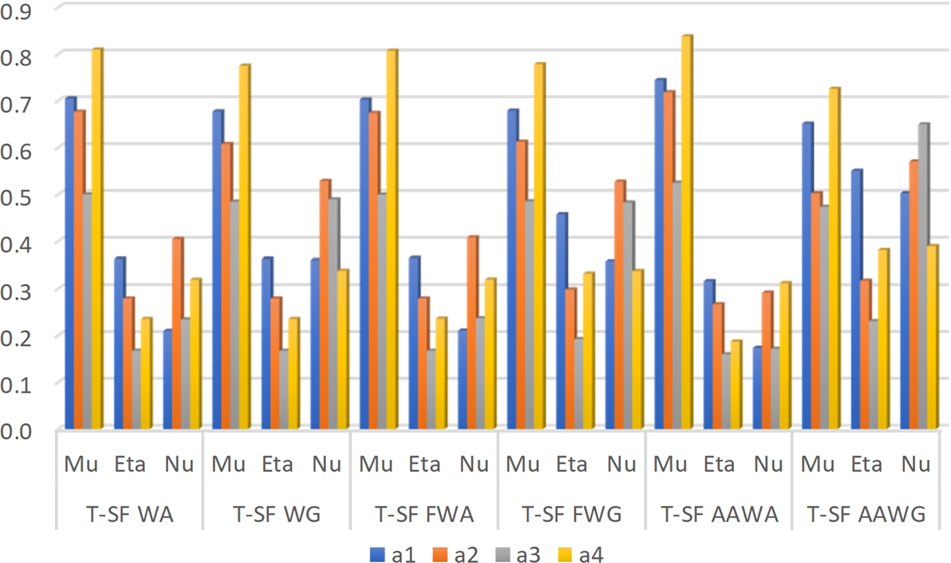
Fig. 4
Juxtaposition of three components of positive-, neutral-, and negative-membership in ${t^{\prime }_{i}}$.
In the light of the location selection issue of a construction company for building new apartments, this research exploited Eqs. (
14)–(
19) to produce the T-SF comprehensive evaluation value
${t^{\prime }_{i}}$, and the determination outcomes are displayed in Table
5. Herein, referring to the specifications by Mahnaz
et al. (
2022) and Hussain
et al. (
2022b), the two parameters
ϕ and Φ were designated as
$\phi =2$ in Eqs. (
15) and (
18) and
$\Phi =5$ in Eqs. (
16) and (
19). To get a general idea of the obtained T-SF comprehensive evaluation values, the juxtaposition results of the three components of positive-, neutral-, and negative-membership (i.e.
${\mu ^{\prime }_{i}}$,
${\eta ^{\prime }_{i}}$, and
${\nu ^{\prime }_{i}}$, respectively) contained in
${t^{\prime }_{i}}$ are sketched in Fig.
4.
Next, this study used Eq. (
20) to generate the aggregated score value
$AS({t^{\prime }_{i}})$ and then identify the corresponding prioritization ranking order, as revealed in Table
6. Over and above that, to conduct a baseline analysis, the technique using the T-SF GGHG operator evolved by Chen
et al. (
2021) will be exploited to be a beginning point used for comparisons. The aggregated score values generated by the T-SF GGHG operator are exhibited in Table
6. As described in the previous subsection, when employing the propounded methodology in this study, the T-SF comprehensive correlation indices (
${\textit{CI}_{\surd }}({a_{i}})$ and
${\textit{CI}_{\wedge }}({a_{i}})$ based on the square root and maximum functions, respectively) are also displayed in Table
6. Moreover, the numbers in parentheses are the orders of precedence for each choice option. The techniques using the T-SF WA, WG, FWA, and FWG operators generated the identical prioritization ranking
${a_{4}}\succ {a_{1}}\succ {a_{3}}\succ {a_{2}}$. The techniques using the T-SF AAWA and GGHG operators and the current multiple-criteria choice method using the square root and maximum functions generated the same prioritization ranking
${a_{4}}\succ {a_{1}}\succ {a_{2}}\succ {a_{3}}$. The use of the technique using the T-SF AAWG operator yielded a particularly different ordering result
${a_{4}}\succ {a_{2}}\succ {a_{1}}\succ {a_{3}}$. Of all the comparative approaches, only the solution results yielded by the T-SF AAWA operator and the current methodology ranked the same as the benchmark method using the T-SF GGHG operator. The Spearman correlation between the benchmark ranking (i.e.
${a_{4}}\succ {a_{1}}\succ {a_{2}}\succ {a_{3}}$) and the solution outcome based on the T-SF WA, WG, FWA, and FWG operators is equal to 0.8. The Spearman correlation between the benchmark ranking and the solution outcome based on the T-SF AAWG operator is also equal to 0.8. It is noted that the Spearman correlation between the two prioritization rankings
${a_{4}}\succ {a_{1}}\succ {a_{3}}\succ {a_{2}}$ and
${a_{4}}\succ {a_{2}}\succ {a_{1}}\succ {a_{3}}$ reduces to 0.4.
Table 6
The aggregated score value and the T-SF comprehensive correlation index with their rank orders.
| Source of methods |
Comparative approach |
${a_{1}}$ |
${a_{2}}$ |
${a_{3}}$ |
${a_{4}}$ |
| Ullah et al. (2020b) |
T-SF WA operator |
0.7252 (2) |
0.6520 (4) |
0.6991 (3) |
0.8091 (1) |
|
T-SF WG operator |
0.6397 (2) |
0.4664 (4) |
0.5001 (3) |
0.7768 (1) |
| Mahnaz et al. (2022) |
T-SF FWA operator |
0.7224 (2) |
0.6472 (4) |
0.6982 (3) |
0.8074 (1) |
|
T-SF FWG operator |
0.5550 (2) |
0.4624 (4) |
0.5048 (3) |
0.7355 (1) |
| Hussain et al. (2022b) |
T-SF AAWA operator |
0.7855 (2) |
0.7575 (3) |
0.7245 (4) |
0.8423 (1) |
|
T-SF AAWG operator |
0.2675 (3) |
0.3334 (2) |
0.1994 (4) |
0.6316 (1) |
| Chen et al. (2021) |
T-SF GGHG operator |
0.4620 (2) |
0.3257 (3) |
0.1951 (4) |
0.6322 (1) |
| Current paper |
Square root function type |
0.7040 (2) |
0.2360 (3) |
0.1801 (4) |
0.9402 (1) |
|
Maximum function type |
0.7157 (2) |
0.2478 (3) |
0.1339 (4) |
0.9578 (1) |
The aggregated score values and T-SF comprehensive correlation indices yielded by the T-SF averaging aggregation operations and the evolved multiple-criteria choice method, respectively, are contrasted in Fig.
5. In particular, Fig.
5(a) reveals the comparisons among the four choice options under distinct comparative approaches. Furthermore, consider that the choice option
${a_{4}}$ performed the best among all comparative approaches, while the choice option
${a_{3}}$ performed the worst among most comparative approaches (i.e. the T-SF AAWA, AAWG, GGHG operators, and the current method based on the square root and maximum functions). The relative performances associated with the best and comparatively worst choice options (i.e.
${a_{4}}$ and
${a_{3}}$, respectively) are contrasted in Fig.
5(b) to highlight their juxtaposition.
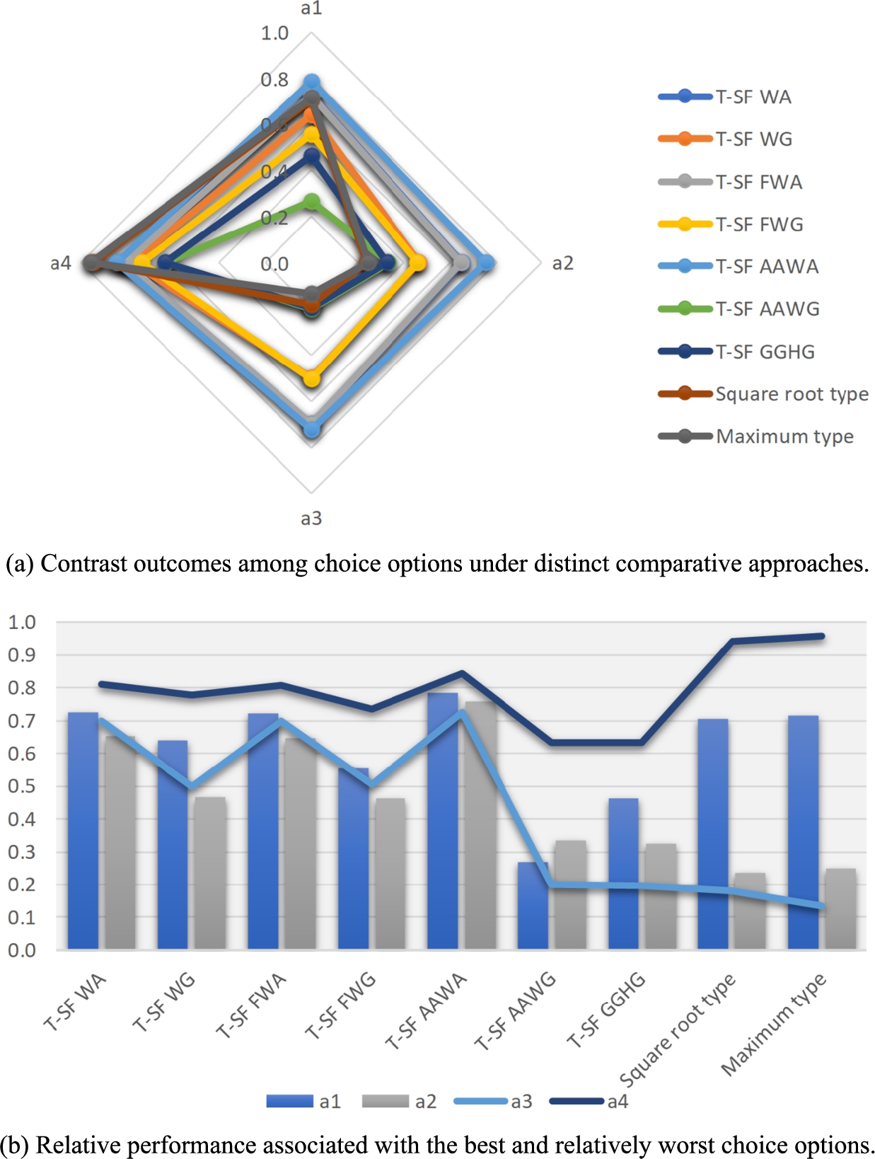
Fig. 5
Comparison results of the aggregated score values/T-SF comprehensive correlation indices.
Going a step further, this study attempts to examine the solution outcomes produced by the comparative approaches with a benchmark ranking by Chen
et al. (
2021). The prioritization ranking (i.e.
${a_{4}}\succ {a_{1}}\succ {a_{3}}\succ {a_{2}}$) obtained by the techniques using the T-SF WA, WG, FWA, and FWG operators differs from the benchmark ranking (i.e.
${a_{4}}\succ {a_{1}}\succ {a_{2}}\succ {a_{3}}$) based on the T-SF GGHG operator in the outranking relationship between
${a_{2}}$ and
${a_{3}}$. The difference between the prioritization ranking (i.e.
${a_{4}}\succ {a_{2}}\succ {a_{1}}\succ {a_{3}}$) rendered by the technique using the T-SF AAWG operator and the benchmark ranking based on the T-SF GGHG operator lies in the outranking relationship between
${a_{1}}$ and
${a_{2}}$. Different from the techniques using the aggregation operators initiated by Ullah
et al. (
2020a), Mahnaz
et al. (
2022), and Hussain
et al. (
2022b), the prioritization rankings yielded by the two approaches based on square root and maximum functions in this study are consistent with the benchmark ranking determined from the T-SF GGHG operator. Therefore, the comparative investigation of the application outcomes supports the superiority of the proposed multiple-criteria choice method grounded in T-SF data-driven correlation measures.
4.3 More Comparative Discussion Based on Parametric Analysis
This subsection has the objective of conducting a comprehensive comparative analysis from a problem-oriented point of view. In the first comparative study, different settings of the anchoring parameter are explored and the yielded outcomes of T-SF comprehensive correlation indices under each scenario are discussed holistically. In the second comparative study, the best and worst choice options that are constituted by the universal and null T-SF sets are replaced by the positive and negative ideal schemes, respectively, to be a benchmark for exploring the effects on the T-SF correlation-focused measurements.
The first comparative study gives thought to distinct assigned values of the anchoring parameter
ξ and investigates the yielded consequences of T-SF comprehensive correlation indices under various parameter settings. By conducting such a comparative study, the effect of the distinct controlling or deciding of the parameter
ξ on the T-SF comprehensive correlation indices
${\textit{CI}_{\surd }}({a_{i}})$ (based on the square root function) and
${\textit{CI}_{\wedge }}({a_{i}})$ (based on the maximum function) can be obtained; moreover, the stability and controllability of the prioritization ranking results can be investigated. In the comparative analysis, the values of the anchoring parameter
ξ were set to 0.0, 0.1, …, 1.0. The juxtaposition and comparisons of
${\textit{CI}_{\surd }}({a_{i}})$ and
${\textit{CI}_{\wedge }}({a_{i}})$ for distinct values of
ξ are portrayed in Fig.
6(a) and Fig.
6(b), respectively.
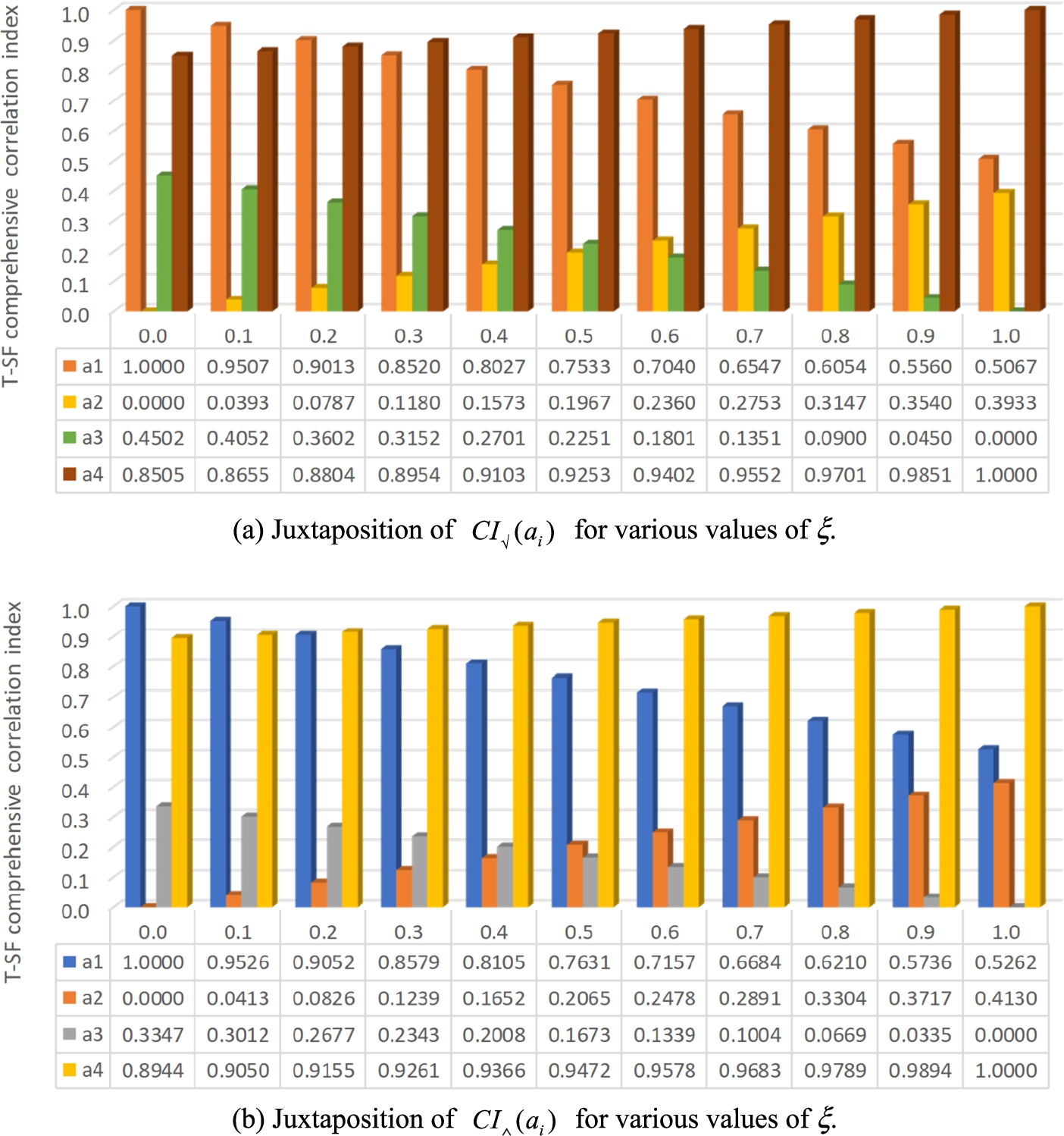
Fig. 6
Contrasts of the T-SF comprehensive correlation indices in distinct settings of the anchoring parameter.
As depicted in Fig.
6(a), the three prioritization rankings
${a_{1}}{\succ _{\surd }}{a_{4}}{\succ _{\surd }}{a_{3}}{\succ _{\surd }}{a_{2}}$,
${a_{4}}{\succ _{\surd }}{a_{1}}{\succ _{\surd }}{a_{3}}{\succ _{\surd }}{a_{2}}$, and
${a_{4}}{\succ _{\surd }}{a_{1}}{\succ _{\surd }}{a_{2}}{\succ _{\surd }}{a_{3}}$ were generated when
$\xi =0.0$, 0.1, 0.2,
$\xi =0.3$, 0.4, 0.5, and
$\xi =0.6,0.7,\dots ,1.0$, respectively. As revealed in Fig.
6(b), the rankings
${a_{1}}{\succ _{\wedge }}{a_{4}}{\succ _{\wedge }}{a_{3}}{\succ _{\wedge }}{a_{2}}$,
${a_{4}}{\succ _{\wedge }}{a_{1}}{\succ _{\wedge }}{a_{3}}{\succ _{\wedge }}{a_{2}}$, and
${a_{4}}{\succ _{\wedge }}{a_{1}}{\succ _{\wedge }}{a_{2}}{\succ _{\wedge }}{a_{3}}$ were produced when
$\xi =0.0,0.1$,
$\xi =0.2,0.3,0.4$, and
$\xi =0.5,0.6,\dots ,1.0$, respectively. In this respect, the prioritization ranking outcomes using the square root function were not much different from those using the maximum function. The main discrimination was that the ranking outcomes in the case of
$\xi =0.2$ and
$\xi =0.5$ are inconsistent. On the other hand, it is worth mentioning that the obtained
${\textit{CI}_{\surd }}({a_{i}})$ and
${\textit{CI}_{\wedge }}({a_{i}})$ values gave rise to identical rankings (i.e. the prioritization rankings
${a_{4}}{\succ _{\surd }}{a_{1}}{\succ _{\surd }}{a_{2}}{\succ _{\surd }}{a_{3}}$ and
${a_{4}}{\succ _{\wedge }}{a_{1}}{\succ _{\wedge }}{a_{2}}{\succ _{\wedge }}{a_{3}}$ when
$\xi =0.6,0.7,\dots ,1.0$ and
$\xi =0.5,0.6,\dots ,1.0$, respectively) in comparison to the ranking outcome rendered by Chen
et al. (
2021). Thus, the efficacy and reasonableness of the proposed methodology can be corroborated because of consistent ranking results in most cases. Furthermore, somewhat different rankings
${a_{4}}{\succ _{\surd }}{a_{1}}{\succ _{\surd }}{a_{3}}{\succ _{\surd }}{a_{2}}$ (based on the square root function) and
${a_{4}}{\succ _{\wedge }}{a_{1}}{\succ _{\wedge }}{a_{3}}{\succ _{\wedge }}{a_{2}}$ (based on the maximum function) were acquired when
$\xi =0.3,0.4,0.5$ and
$\xi =0.2,0.3,0.4$, respectively. Nonetheless, different outcomes were yielded in face of the small values of
ξ, namely
${a_{1}}{\succ _{\surd }}{a_{4}}{\succ _{\surd }}{a_{3}}{\succ _{\surd }}{a_{2}}$ and
${a_{1}}{\succ _{\wedge }}{a_{4}}{\succ _{\wedge }}{a_{3}}{\succ _{\wedge }}{a_{2}}$ when
$\xi =0.0,0.1,0.2$ and
$\xi =0.0,0.1$, respectively. Overall, stable and justified consequences can be generated under most settings of
ξ. When
$\xi =0.0,0.1,0.2$ based on the “square root function” type or
$\xi =0.0,0.1$ based on the “maximum function” type, distinct prioritization ranking outcomes can be rendered to reflect the change of the
ξ values, which gives substance to the pliability of the current methods by adjusting the anchoring parameter
ξ. The comparison consequence demonstrates that by controlling the parameter values, stable and flexible prioritization rankings can be produced by using the propounded methodology.
In the second comparative study, the best choice option ${a_{+}}$ and the worst choice option ${a_{-}}$ (composed of the universal T-SF set and the null T-SF set) are replaced by the positive and negative ideal schemes, respectively, as an alternate benchmark for calculating the T-SF correlation-focused measurements. To accommodate the change of the reference points, this study would like to yield the corresponding T-SF correlation-focused measurements, so that the subsequent practical data processing and multiple-criteria evaluation procedures can operate smoothly. Through the juxtaposition and comparison of the solution outcomes, the influence of distinct points of reference on the yielded results can be clarified. Moreover, through the side-by-side comparison, the advantages of taking ${a_{+}}$ and ${a_{-}}$ as points of reference can be demonstrated and justified.
The positive and negative ideal schemes would be exploited to replace the best and worst choice options, respectively, to explore the influences of different points of reference on the T-SF correlation-focused measurements and resolution consequences. More specifically, instead of the universal and null T-SF sets, the T-SF characteristics of the ideal schemes would be established using the union and intersection operations. Let ${a_{\ast }}$ indicate the positive ideal scheme, where the T-SF characteristic ${T_{\ast }}=\{\langle {c_{j}},{t_{\ast j}}\rangle \hspace{0.1667em}|\hspace{0.1667em}{c_{j}}\in C\}=\{\langle {c_{j}},({\mu _{\ast j}},{\eta _{\ast j}},{\nu _{\ast j}})\rangle \hspace{0.1667em}|\hspace{0.1667em}{c_{j}}\in C\}$. Let ${a_{\mathrm{\# }}}$ signify the negative ideal scheme, where the T-SF characteristic ${T_{\mathrm{\# }}}=\{\langle {c_{j}},{t_{\mathrm{\# }j}}\rangle \hspace{0.1667em}|\hspace{0.1667em}{c_{j}}\in C\}=\{\langle {c_{j}},({\mu _{\mathrm{\# }j}},{\eta _{\mathrm{\# }j}},{\nu _{\mathrm{\# }j}})\rangle \hspace{0.1667em}|\hspace{0.1667em}{c_{j}}\in C\}$. Utilizing the set operations ∪ and ∩, ${T_{\ast }}$ and ${T_{\mathrm{\# }}}$ are delineated in this fashion:
-
1. $\begin{array}[t]{r@{\hskip4.0pt}c@{\hskip4.0pt}l}{T_{\ast }}& =& \Big\{\Big\langle {c_{j}},\Big({\max _{i=1}^{m}}{\mu _{ij}},{\min _{i=1}^{m}}{\eta _{ij}},{\min _{i=1}^{m}}{\nu _{ij}}\Big)\Big\rangle \hspace{0.1667em}\Big|\hspace{0.1667em}{c_{j}}\in {C_{\textit{Po}}},\\ {} & & \Big\langle {c_{j}},\Big({\min _{i=1}^{m}}{\mu _{ij}},{\min _{i=1}^{m}}{\eta _{ij}},{\max _{i=1}^{m}}{\nu _{ij}}\Big)\Big\rangle \hspace{0.1667em}\Big|\hspace{0.1667em}{c_{j}}\in {C_{\textit{Ne}}}\Big\};\end{array}$
-
2. $\begin{array}[t]{r@{\hskip4.0pt}c@{\hskip4.0pt}l}{T_{\mathrm{\# }}}& =& \Big\{\Big\langle {c_{j}},\Big({\min _{i=1}^{m}}{\mu _{ij}},{\min _{i=1}^{m}}{\eta _{ij}},{\max _{i=1}^{m}}{\nu _{ij}}\Big)\Big\rangle \hspace{0.1667em}\Big|\hspace{0.1667em}{c_{j}}\in {C_{\textit{Po}}},\\ {} & & \Big\langle {c_{j}},\Big({\max _{i=1}^{m}}{\mu _{ij}},{\min _{i=1}^{m}}{\eta _{ij}},{\min _{i=1}^{m}}{\nu _{ij}}\Big)\Big\rangle \hspace{0.1667em}\Big|\hspace{0.1667em}{c_{j}}\in {C_{\textit{Ne}}}\Big\}.\end{array}$
Recall that
${C_{\textit{Po}}}=\{{c_{2}},{c_{3}}\}$ and
${C_{\textit{Ne}}}=\{{c_{1}},{c_{4}}\}$ in the location selection problem. Using the aforesaid manner, the T-SF characteristics of
${a_{\ast }}$ and
${a_{\mathrm{\# }}}$ were identified as follows:
${T_{\ast }}=\{\langle {c_{1}},(0.14,0.12,0.83)\rangle ,\langle {c_{2}},(0.91,0.12,0.13)\rangle ,\langle {c_{3}},(0.81,0.11,0.11)\rangle ,\langle {c_{4}},(0.11,0.14,0.84)\rangle \}$ and
${T_{\mathrm{\# }}}=\{\langle {c_{1}},(0.75,0.12,0.41)\rangle ,\langle {c_{2}},(0.26,0.12,0.63)\rangle ,\langle {c_{3}},(0.56,0.11,0.55)\rangle ,\langle {c_{4}},(0.61,0.14,0.45)\rangle \}$. The corresponding T-SF weighted characteristics were given by:
${T_{\ast }^{W}}=\{\langle {c_{1}},(0.1300,0.1156,0.8012)\rangle ,\langle {c_{2}},(0.7542,0.1171,0.1009)\rangle ,\langle {c_{3}},(0.8422,0.1147,0.1060)\rangle ,\langle {c_{4}},(0.1286,0.1637,0.8922)\rangle \}$ and
${T_{\mathrm{\# }}^{W}}=\{\langle {c_{1}},(0.7080,0.1156,0.3965)\rangle ,\langle {c_{2}},(0.1919,0.1171,0.5083)\rangle ,\langle {c_{3}},(0.5914,0.1147,0.5538)\rangle ,\langle {c_{4}},(0.6963,0.1637,0.5210)\rangle \}$. The T-SF weighted informational energies were derived as:
$\textit{IE}({T_{\ast }^{W}})=2.1053$ and
$\textit{IE}({T_{\mathrm{\# }}^{W}})=2.0837$. The comparisons of the T-SF weighted correlation functions
$\textit{CF}({T_{i}^{W}},{T_{+}^{W}})$,
$\textit{CF}({T_{i}^{W}},{T_{\ast }^{W}})$,
$\textit{CF}({T_{i}^{W}},{T_{-}^{W}})$, and
$\textit{CF}({T_{i}^{W}},{T_{\mathrm{\# }}^{W}})$ are manifested in Fig.
7. Furthermore, the T-SF weighted correlation coefficients
${\textit{CC}_{\surd }}({T_{i}^{W}},{T_{+}^{W}})$,
${\textit{CC}_{\surd }}({T_{i}^{W}},{T_{\ast }^{W}})$,
${\textit{CC}_{\surd }}({T_{i}^{W}},{T_{-}^{W}})$, and
${\textit{CC}_{\surd }}({T_{i}^{W}},{T_{\mathrm{\# }}^{W}})$ are contrasted in Fig.
8(a), while the comparisons of
${\textit{CC}_{\wedge }}({T_{i}^{W}},{T_{+}^{W}})$,
${\textit{CC}_{\wedge }}({T_{i}^{W}},{T_{\ast }^{W}})$,
${\textit{CC}_{\wedge }}({T_{i}^{W}},{T_{-}^{W}})$, and
${\textit{CC}_{\wedge }}({T_{i}^{W}},{T_{\mathrm{\# }}^{W}})$ are exhibited in Fig.
8(b).
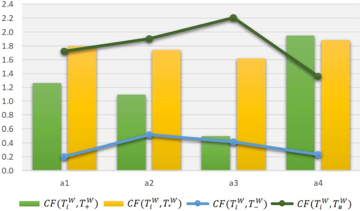
Fig. 7
Contrast outcomes of the T-SF weighted correlation functions concerning distinct points of reference.
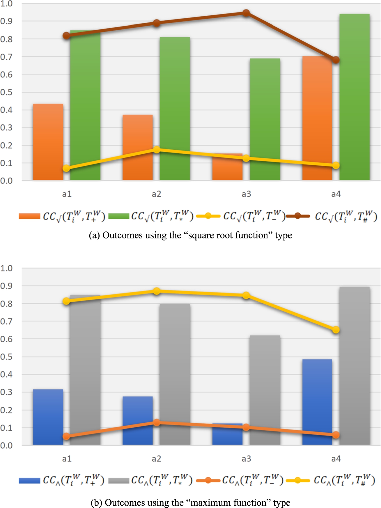
Fig. 8
Contrast outcomes of the T-SF weighted correlation coefficients concerning distinct points of reference. (a) Outcomes using the “square root function” type. (b) Outcomes using the “maximum function” type.
First, consider the contrast outcomes of the T-SF weighted correlation functions concerning the best choice option
${a_{+}}$ and the positive ideal scheme
${a_{\ast }}$, as revealed in Fig.
5. The differences among the
$\textit{CF}({T_{i}^{W}},{T_{+}^{W}})$ values of the four choice options (
${a_{1}}-{a_{4}}$) were significantly higher than the differences among the
$\textit{CF}({T_{i}^{W}},{T_{\ast }^{W}})$ values. In particular, the gap between the maximum value (i.e.
$\textit{CF}({T_{4}^{W}},{T_{+}^{W}})$) and the minimum value (i.e.
$\textit{CF}({T_{3}^{W}},{T_{+}^{W}})$) was quite pronounced. However, the gap between the maximum value (i.e.
$\textit{CF}({T_{4}^{W}},{T_{\ast }^{W}})$) and the minimum value (i.e.
$\textit{CF}({T_{3}^{W}},{T_{\ast }^{W}})$) did not show a particularly significant difference. Next, concerning the T-SF weighted correlation functions toward the worst choice option
${a_{-}}$ and the negative ideal scheme
${a_{\mathrm{\# }}}$, the maximum value of
$\textit{CF}({T_{i}^{W}},{T_{-}^{W}})$ and the maximum value of
$\textit{CF}({T_{i}^{W}},{T_{\mathrm{\# }}^{W}})$ correspond to different options; the same is true for the minimum value of
$\textit{CF}({T_{i}^{W}},{T_{-}^{W}})$ (or
$\textit{CF}({T_{i}^{W}},{T_{\mathrm{\# }}^{W}})$). To be precise, the options
${a_{2}}$ and
${a_{1}}$ enjoy the largest and smallest values, respectively, of
$\textit{CF}({T_{i}^{W}},{T_{-}^{W}})$;
${a_{3}}$ and
${a_{4}}$ enjoy the largest and smallest values, respectively, of
$\textit{CF}({T_{i}^{W}},{T_{\mathrm{\# }}^{W}})$.
Next, consider the comparisons of the T-SF weighted correlation coefficients with relevance to two types of points of reference (i.e. one type for the best and worst choice options and the other type for the positive and negative ideal schemes). Let us investigate the contrast outcomes in Fig.
8(a) using the “square root function” type. The
${\textit{CC}_{\surd }}({T_{i}^{W}},{T_{\ast }^{W}})$ values of the four choice options were significantly higher than the
${\textit{CC}_{\surd }}({T_{i}^{W}},{T_{+}^{W}})$ values; this phenomenon was also found in the comparisons of the values of
${\textit{CC}_{\surd }}({T_{i}^{W}},{T_{\mathrm{\# }}^{W}})$ and
${\textit{CC}_{\surd }}({T_{i}^{W}},{T_{-}^{W}})$. The higher the value of
${\textit{CC}_{\surd }}({T_{i}^{W}},{T_{+}^{W}})$ (or
${\textit{CC}_{\surd }}({T_{i}^{W}},{T_{\ast }^{W}})$), the higher the correlation between the corresponding option
${a_{i}}$ and
${a_{+}}$ (or
${a_{\ast }}$). Accordingly, the decision-maker expects to choose the option that is highly correlated with the best choice option (or the positive ideal scheme). The lower the value of
${\textit{CC}_{\surd }}({T_{i}^{W}},{T_{-}^{W}})$ (or
${\textit{CC}_{\surd }}({T_{i}^{W}},{T_{\mathrm{\# }}^{W}})$), the lower the correlation between
${a_{i}}$ and
${a_{-}}$ (or
${a_{\mathrm{\# }}}$). In this regard, the decision-maker expects to choose the option that lowly correlates with the worst choice option (or the negative ideal scheme). In Fig.
8(a), the numerical orders of the T-SF weighted correlation coefficients for mutual relationships with
${a_{+}}$ and
${a_{\ast }}$ were
${\textit{CC}_{\surd }}({T_{4}^{W}},{T_{+}^{W}})>{\textit{CC}_{\surd }}({T_{1}^{W}},{T_{+}^{W}})>{\textit{CC}_{\surd }}({T_{2}^{W}},{T_{+}^{W}})>{\textit{CC}_{\surd }}({T_{3}^{W}},{T_{+}^{W}})$ and
${\textit{CC}_{\surd }}({T_{4}^{W}},{T_{\ast }^{W}})>{\textit{CC}_{\surd }}({T_{1}^{W}},{T_{\ast }^{W}})>{\textit{CC}_{\surd }}({T_{2}^{W}},{T_{\ast }^{W}})>{\textit{CC}_{\surd }}({T_{3}^{W}},{T_{\ast }^{W}})$, respectively. Different from the identical ranking orders above, the numerical orders of the T-SF weighted correlation coefficients for mutual relationships with
${a_{-}}$ and
${a_{\mathrm{\# }}}$ were
${\textit{CC}_{\surd }}({T_{1}^{W}},{T_{-}^{W}})<{\textit{CC}_{\surd }}({T_{4}^{W}},{T_{-}^{W}})<{\textit{CC}_{\surd }}({T_{3}^{W}},{T_{-}^{W}})<{\textit{CC}_{\surd }}({T_{2}^{W}},{T_{-}^{W}})$ and
${\textit{CC}_{\surd }}({T_{4}^{W}},{T_{\mathrm{\# }}^{W}})<{\textit{CC}_{\surd }}({T_{1}^{W}},{T_{\mathrm{\# }}^{W}})<{\textit{CC}_{\surd }}({T_{2}^{W}},{T_{\mathrm{\# }}^{W}})<{\textit{CC}_{\surd }}({T_{3}^{W}},{T_{\mathrm{\# }}^{W}})$, respectively. In Fig.
8(b), the findings concerning the contrast outcomes using the “maximum function” type were about the same as those using the “square root function” type except for the results of
${\textit{CC}_{\wedge }}({T_{i}^{W}},{T_{\mathrm{\# }}^{W}})$. Specifically, the numerical orders of
${\textit{CC}_{\wedge }}({T_{i}^{W}},{T_{\mathrm{\# }}^{W}})$ were given by
${\textit{CC}_{\wedge }}({T_{4}^{W}},{T_{\mathrm{\# }}^{W}})<{\textit{CC}_{\wedge }}({T_{1}^{W}},{T_{\mathrm{\# }}^{W}})<{\textit{CC}_{\wedge }}({T_{3}^{W}},{T_{\mathrm{\# }}^{W}})<{\textit{CC}_{\wedge }}({T_{2}^{W}},{T_{\mathrm{\# }}^{W}})$. In the matter of the numerical orders of the T-SF weighted correlation coefficients among the four options, the two ranking outcomes employing
${\textit{CC}_{\surd }}({T_{i}^{W}},{T_{+}^{W}})$ and
${\textit{CC}_{\surd }}({T_{i}^{W}},{T_{\ast }^{W}})$ were consistent; however, the two ranking outcomes via
${\textit{CC}_{\surd }}({T_{i}^{W}},{T_{-}^{W}})$ and
${\textit{CC}_{\surd }}({T_{i}^{W}},{T_{\mathrm{\# }}^{W}})$ were somewhat different. To unify the inconsistent numerical orders, this study continued to calculate the T-SF comprehensive correlation indices for the final decision.
To facilitate discussing the effects of the anchoring parameter
ξ regarding the solution consequences, this study set eleven different values for the parameter to calculate the T-SF comprehensive correlation indices and identify the ultimate ranking outcome under various scenarios. This study designated the anchoring parameter
ξ ranging from 0 to 1, wherein
$\xi =0.0,0.1,\dots ,1.0$. Let
$\underline{\textit{CC}}{\hspace{0.1667em}_{\surd }^{\ast }}={\min _{{i^{\prime }}=1}^{4}}{\textit{CC}_{\surd }}({T_{{i^{\prime }}}^{W}},{T_{\ast }^{W}})$,
$\overline{\textit{CC}}{\hspace{0.1667em}_{\surd }^{\ast }}={\max _{{i^{\prime }}=1}^{4}}{\textit{CC}_{\surd }}({T_{{i^{\prime }}}^{W}},{T_{\ast }^{W}}$),
$\underline{\textit{CC}}{\hspace{0.1667em}_{\surd }^{\mathrm{\# }}}={\min _{{i^{\prime }}=1}^{4}}{\textit{CC}_{\surd }}({T_{{i^{\prime }}}^{W}},{T_{\mathrm{\# }}^{W}})$, and
$\overline{\textit{CC}}{\hspace{0.1667em}_{\surd }^{\mathrm{\# }}}={\max _{{i^{\prime }}=1}^{4}}\hspace{-0.1667em}{\textit{CC}_{\surd }}({T_{{i^{\prime }}}^{W}},{T_{\mathrm{\# }}^{W}})$ for the “square root function” type. Let
$\underline{\textit{CC}}{\hspace{0.1667em}_{\wedge }^{\ast }}\hspace{-0.1667em}=\hspace{-0.1667em}{\min _{{i^{\prime }}=1}^{4}}{\textit{CC}_{\wedge }}({T_{{i^{\prime }}}^{W}},{T_{\ast }^{W}})$,
$\overline{\textit{CC}}{\hspace{0.1667em}_{\wedge }^{\ast }}={\max _{{i^{\prime }}=1}^{4}}{\textit{CC}_{\wedge }}({T_{{i^{\prime }}}^{W}},{T_{\ast }^{W}})$,
$\underline{\textit{CC}}{\hspace{0.1667em}_{\wedge }^{\mathrm{\# }}}={\min _{{i^{\prime }}=1}^{4}}{\textit{CC}_{\wedge }}({T_{{i^{\prime }}}^{W}},{T_{\mathrm{\# }}^{W}})$, and
$\overline{\textit{CC}}{\hspace{0.1667em}_{\wedge }^{\mathrm{\# }}}={\max _{{i^{\prime }}=1}^{4}}{\textit{CC}_{\wedge }}({T_{{i^{\prime }}}^{W}},{T_{\mathrm{\# }}^{W}})$ for the “maximum function” type. On the grounds of the ideal schemes
${a_{\ast }}$ and
${a_{\mathrm{\# }}}$, the T-SF comprehensive correlation indices
${\textit{CI}^{\prime }_{\surd }}({a_{i}})$ and
${\textit{CI}^{\prime }_{\wedge }}({a_{i}})$ are elucidated in this fashion:
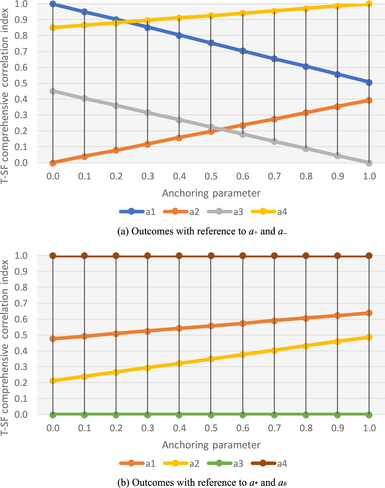
Fig. 9
Contrast outcomes of ${\textit{CI}_{\surd }}({a_{i}})$ and ${\textit{CI}^{\prime }_{\surd }}({a_{i}})$ for various values of ξ.
Regarding the “square root function” type, the juxtaposition of the T-SF comprehensive correlation indices
${\textit{CI}_{\surd }}({a_{i}})$ and
${\textit{CI}^{\prime }_{\surd }}({a_{i}})$ for various values of
ξ are displayed in Fig.
9. Specifically, Fig.
9(a) reveals the contrast outcomes concerning the points of reference
${a_{+}}$ and
${a_{-}}$, while Fig.
9(b) demonstrates the comparisons in connection with the points of reference
${a_{\ast }}$ and
${a_{\mathrm{\# }}}$. For the “maximum function” type, the juxtaposition of the T-SF comprehensive correlation indices
${\textit{CI}_{\surd }}({a_{i}})$ and
${\textit{CI}^{\prime }_{\surd }}({a_{i}})$ for various values of
ξ are sketched in Fig.
10. Herein, Fig.
10(a) shows the comparison consequence on the grounds of
${a_{+}}$ and
${a_{-}}$, while Fig.
10(b) exemplifies the contrasts based on
${a_{\ast }}$ and
${a_{\mathrm{\# }}}$.
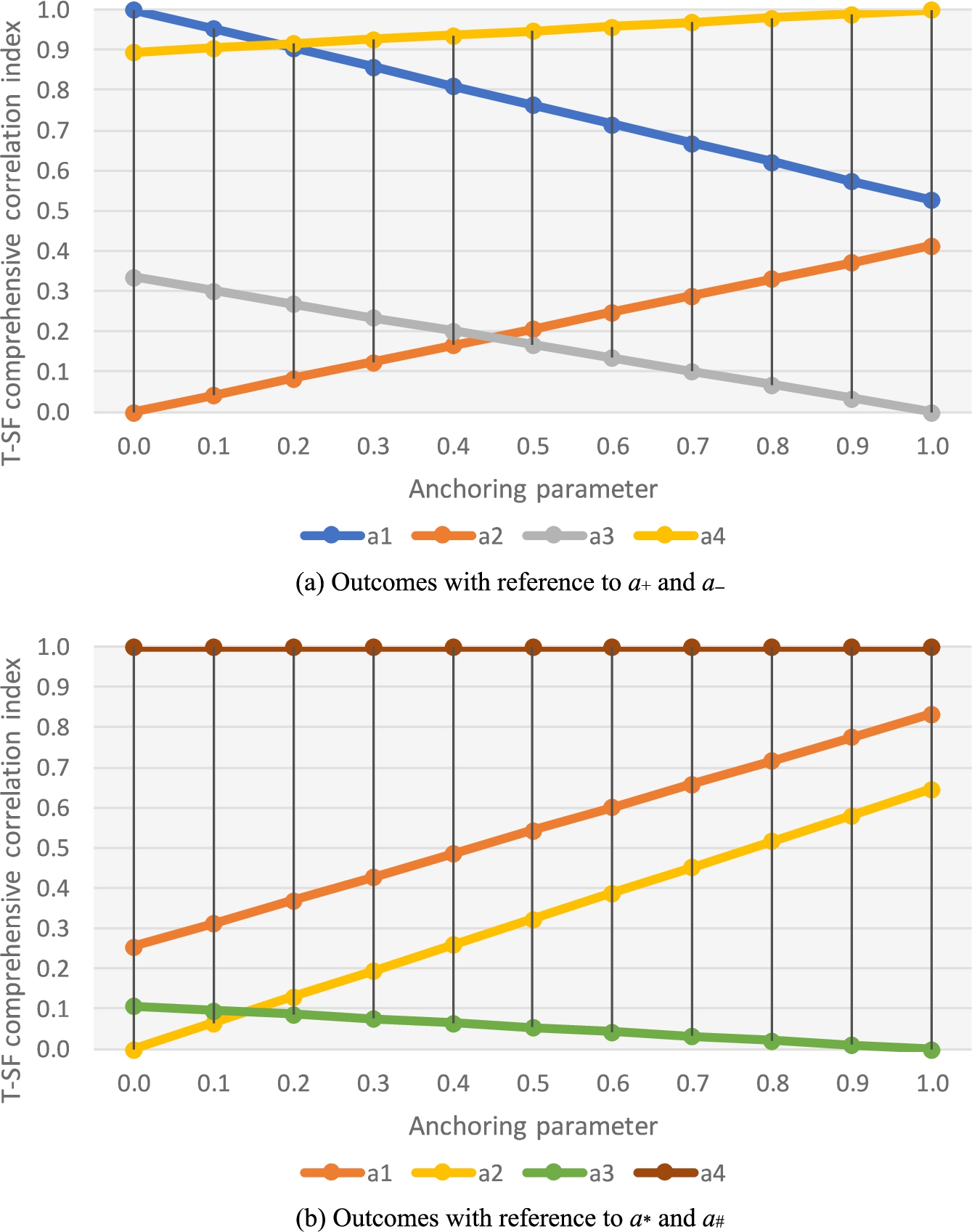
Fig. 10
Contrast outcomes of ${\textit{CI}_{\wedge }}({a_{i}})$ and ${\textit{CI}^{\prime }_{\wedge }}({a_{i}})$ for various values of ξ.
On the grounds of the reference points of the ideal schemes
${a_{\ast }}$ and
${a_{\mathrm{\# }}}$, the contrast outcomes of the T-SF comprehensive correlation indices among the four options presented moderately unreasonable patterns; moreover, these results may be difficult to be accepted by the decision-maker. To be specific, the unusual consequences were produced using the “square root function” type, i.e.
${\textit{CI}^{\prime }_{\surd }}({a_{3}})=0$ and
${\textit{CI}^{\prime }_{\surd }}({a_{4}})=1$ for all
$\xi =0.0,0.1,\dots ,1.0$, as displayed in Fig.
9(b). Additionally, it was received that
${\textit{CI}^{\prime }_{\wedge }}({a_{4}})=1$ predicated on the “maximum function” type for all
$\xi =0.0,0.1,\dots ,1.0$, as displayed in Fig.
10(b). Regardless of how the value of the anchoring parameter
ξ changed, the indices
${\textit{CI}^{\prime }_{\surd }}({a_{3}})$,
${\textit{CI}^{\prime }_{\surd }}({a_{4}})$, and
${\textit{CI}^{\prime }_{\wedge }}({a_{4}})$ were fixed at 0, 1, and 1, respectively. These findings revealed that the multiple-criteria analysis approach that exploited the positive and negative ideal schemes as a benchmark for reference was not sensitive enough to reflect changes in various
ξ values. On the contrary, the propounded methodology predicated on the best and worst choice options (i.e.
${a_{+}}$ and
${a_{-}}$) that were established on the universal and null T-SF sets generated reasonable and desirable consequences.

