1 Introduction
Fuzzy Sets theory, developed by Zadeh (1965), is a useful and appropriate approach to deal with imprecise and uncertain information in ambiguous situations (Farrokhizadeh et al., 2021). After introducing fuzzy sets by Zadeh (1965), they have been prevalent in almost all branches of science (Kutlu Gündoğdu and Kahraman, 2019a). Many researchers (Zadeh, 1975; Grattan-Guinness, 1976; Atanassov, 1986; Yager, 1986; Atanassov, 1999; Smarandache, 1998; Torra, 2010; Cu’ò’ng, 2014; Yager, 2017; Gündoğdu and Kahraman, 2019a) have introduced many extensions of ordinary fuzzy sets in the literature. Numerous researchers have utilized these extensions in recent years in the solution of multi-attribute decision-making problems (Gündoğdu and Kahraman, 2019b). These extensions are presented in a chronological order, as given in Fig. 1.
The latest extension of fuzzy sets is Spherical Fuzzy Sets (SFSs), recently developed by Kutlu Gündoğdu and Kahraman (2019a), where the squared sum of hesitancy, membership, and non-membership degrees is at most equal to 1.
The extensions of ordinary fuzzy sets given in Fig. 1 can be classified into two main groups: 1. Intuitionistic fuzzy sets (Atanassov, 1986) and their versions, 2. Neutrosophic sets (Smarandache, 2000) and their versions. The first group extensions can be defined by a membership degree and a non-membership degree, whereas the second group extensions can be defined by a membership degree (truthiness), a non-membership degree (falsity), and a hesitancy degree (indeterminacy). Picture Fuzzy Sets are a particular case of neutrosophic sets and also of refined neutrosophic sets (Smarandache, 2013). The ultimate extension of IFS is q-Rung orthopair fuzzy sets (Yager, 2016), while the ultimate extension of picture fuzzy sets is t-spherical fuzzy sets (Ullah et al., 2018). Spherical fuzzy sets are located between picture fuzzy sets and t-spherical fuzzy sets.
As indicated above, spherical and picture fuzzy sets are in the same group because of the definition of membership functions. The squared sum of membership, non-membership, and hesitancy degrees is equal to or less than 1.0 in spherical fuzzy sets whereas it is valid for the first degree sum in picture fuzzy sets. Pythagorean fuzzy sets are in the other group since the hesitancy degree depends on membership and non-membership degrees. Pythagorean fuzzy sets correspond to spherical fuzzy sets in the other group since the squared sum of the parameters is at most equal to 1 in both extensions (Liu et al., 2019). Ashraf et al. (2019a,2019b) proposed spherical fuzzy sets with some operational rules and aggregation operations based on Archimedean t-norm and t-conorms.
The extensions of ordinary fuzzy sets have an important impact and have been used frequently on the progress of Multiple Attribute Decision-Making (MADM) research area in an uncertain environment (Donyatalab et al., 2019). MADM deals with problems where there are discrete attributes and more alternatives than one for evaluation (Kahraman et al., 2019b). MADM problems include numerous attributes, which are tangible or intangible (Karasan et al., 2019). Group decision making is a type of MADM problems that is usually understood as aggregating different discrete preferences on a given set of alternatives to a single collective preference. Group decision making involves multiple decision-makers, each with different skills, experience, and knowledge related to the problem’s different attributes. This type of problems are known as Multiple-Attribute Group Decision-Making (MAGDM) (Robinson and Amirtharaj, 2015).
Several MADM methods are extended to Spherical Fuzzy Sets, and their applications are investigated in the literature. Mahmood et al. (2019) investigated the medical diagnostics and decision-making problem in the spherical fuzzy environment as a practical application. Zeng et al. (2019), using the SF-TOPSIS methodology, developed a multi-attribute decision-making problem in an SF environment. They adopted a new approach of covering-based spherical fuzzy rough set (CSFRS) models utilizing spherical fuzzy β-neighbourhoods to hybrid spherical fuzzy sets with notions of covering the rough set. In another research, Kutlu Gündoğdu and Kahraman (2019c), Kutlu Gündoğdu et al. (2020) extended the classical (VIKOR) method to the spherical fuzzy VIKOR (SF-VIKOR) method and showed its applicability and validity through a waste management problem. Kahraman et al. (2019b) developed and used the spherical fuzzy TOPSIS method in a hospital location selection problem. The extension of the classical analytic hierarchy process (AHP) to spherical fuzzy AHP (SF-AHP) method and its application to renewable energy location selection is proposed by Kutlu Gündoğdu and Kahraman (2019b). The application of the spherical fuzzy analytic hierarchy process (AHP) method in an industrial robot selection problem has been researched by Kutlu Gündoğdu and Kahraman (2020). The multi-criteria decision-making method TOPSIS is extended to spherical fuzzy TOPSIS in Kutlu Gündoğdu and Kahraman’s (2019c) research. The extensions of traditional WASPAS and CODAS methods to spherical fuzzy WASPAS and CODAS have also been developed by Kutlu Gündoğdu and Kahraman (2019a; 2019b). Kutlu Gündoğdu (2020) developed the spherical fuzzy MULTIMOORA method to efficiently solve complex problems, which require assessment and estimation under an unstable data environment. The interval-valued spherical fuzzy sets are employed in developing the extension of TOPSIS under fuzziness by Kutlu Gündoğdu and Kahraman (2019a). They used the proposed method in solving a multiple criteria selection problems among 3D printers. Liu et al. (2020) proposed an approach based on linguistic spherical fuzzy sets for public evaluation of shared bicycles in China. Kahraman et al. (2020) developed a performance measurement method in order to rank the firms using a spherical fuzzy multi-attribute decision making approach. A new approach to the fuzzy TOPSIS method based on entropy measures using spherical fuzzy information-based decision-making techniques for MAGDM problems was presented by Barukab et al. (2019). Finally, some novel similarity measures in the spherical fuzzy environment have been proposed by Seyfi Shishavan et al. (2020).
As a classical decision analysis method of MCDM, the linear assignment method (LAM) was initially proposed by Bernardo and Blin (1977), inspiring from assignment problem in linear programming for MADM (Razavi Hajiagha et al., 2018). The combination of the criteria-wise rankings into an overall preference ranking that produces an optimal compromise among the several component rankings is the LAM’s basic idea (Liang et al., 2019). In the classical linear assignment method, usually crisp values of decision matrix are used. Considering the inevitable uncertainty of decision-making problems and real-life, LAM is extended under different fuzzy extensions by scholars using different modelling and solving approaches.
Razavi Hajiagha et al. (2018) proposed a method based on a linear assignment method to solve the group decision-making problems using hesitant fuzzy linguistic term sets. The results are compared with other methods to outline the model’s efficiency. An approach to solve the multiple criteria decision making (MCDM) problems under the hesitant fuzzy environment was developed by Wei et al. (2017). The information about the criteria weights are correlative and based on the λ-fuzzy measure. Based on signed distances, Chen (2013) developed a new linear assignment method within the interval type-2 trapezoidal fuzzy numbers framework to produce an optimal preference ranking of the alternatives. In another research, Yang et al. (2018) developed a new multiple attribute decision-making method based on the interval neutrosophic sets and linear assignment. Developing an extended linear assignment method to solve multi-criteria decision-making (MCDM) problems under Pythagorean fuzzy environment was the aim of Liang et al. (2019). A new approach based on a linear assignment method was presented by Bashiri et al. (2011) for selecting the optimum maintenance strategy using qualitative and quantitative data through interaction with the maintenance experts. By extending the traditional linear assignment method, Chen (2014) proposed an efficient method for solving MCDM problems in the interval-valued intuitionistic fuzzy environment. Finally, Liang et al. (2018) developed the linear assignment method for interval-valued Pythagorean fuzzy sets.
Based on the literature and the best of our knowledge, there is no research about the extension and application of the linear assignment method in spherical fuzzy environment. Therefore, this paper aims to develop a novel multi-attribute decision-making method based on a linear assignment approach in spherical fuzzy environment.
In order to achieve this, the following steps will be performed step by step. Section 2 briefly reviews the concepts of spherical fuzzy sets and relative operations and aggregation operators. Section 3 formulates an MCDA problem in which the evaluation of alternatives is expressed by spherical fuzzy sets (SFS). This section also develops an extended linear assignment method for SFS using aggregation operator concepts, the score and accuracy functions, rank frequency matrices, and weighted-rank frequency matrices to determine the rank of the given alternatives. Section 4 demonstrates the feasibility and applicability of the proposed method by applying it to the MCDA problem of wind power farm location selection. This section also consists of a comparative analysis with SF-AHP and SF-WASPAS methods and discusses the proposed method’s advantages with more details. Finally, Section 5 presents the conclusions.
2 Preliminaries
The concept of Spherical Fuzzy Sets (SFS) provides a larger preference domain for decision-makers to assign membership degrees since the squared sum of the spherical parameters is allowed to be at most 1.
Definition 1 (See, Gündoğdu and Kahraman, 2019c).
Single valued Spherical Fuzzy Sets (SFS) ${\tilde{A}_{S}}$ of the universe of discourse X is given by:
where ${\mu _{{\tilde{A}_{s}}}}(u),{\vartheta _{{\tilde{A}_{s}}}}(u),{I_{{\tilde{A}_{s}}}}(u):U\to [0,1]$ are the degrees of membership, non-membership, and indeterminacy of x to ${\tilde{A}_{S}}$, respectively, and:
Then, $\sqrt{1-({\mu _{{\tilde{A}_{s}}}^{2}}(x)+{\vartheta _{{\tilde{A}_{s}}}^{2}}(x)+{I_{{\tilde{A}_{s}}}^{2}}(x))}$ is defined as the refusal degree of x in X.
(1)
\[ {\tilde{A}_{s}}=\big\{x,{\mu _{{\tilde{A}_{s}}}}(x),{\vartheta _{{\tilde{A}_{s}}}}(x),{I_{{\tilde{A}_{s}}}}(x)\hspace{0.1667em}\big|\hspace{0.1667em}x\in X\big\},\](2)
\[ 0\leqslant {\mu _{{\tilde{A}_{s}}}^{2}}(x)+{\vartheta _{{\tilde{A}_{s}}}^{2}}(x)+{I_{{\tilde{A}_{s}}}^{2}}(x)\leqslant 1.\]Definition 2 (See, Gündoğdu and Kahraman, 2019c).
Suppose that ${\tilde{A}_{s}}$ and ${\tilde{B}_{s}}$ be any two Spherical Fuzzy sets. So the basic operations of SFSs can be defined as follow:
Addition
Multiplication
Multiplication by a scalar; $k>0$
Power of ${\tilde{A}_{s}}$; $k>0$
(3)
\[\begin{aligned}{}{\tilde{A}_{s}}\oplus {\tilde{B}_{s}}=& \Big\{\sqrt{{\mu _{{\tilde{A}_{s}}}^{2}}+{\mu _{{\tilde{B}_{s}}}^{2}}-{\mu _{{\tilde{A}_{s}}}^{2}}{\mu _{{\tilde{B}_{s}}}^{2}}},{\vartheta _{{\tilde{A}_{s}}}}{\vartheta _{{\tilde{B}_{s}}}},\\ {} & \sqrt{\big(1-{\mu _{{\tilde{B}_{s}}}^{2}}\big){I_{{\tilde{A}_{s}}}^{2}}+\big(1-{\mu _{{\tilde{A}_{s}}}^{2}}\big){I_{{\tilde{B}_{s}}}^{2}}-{I_{{\tilde{A}_{s}}}^{2}}{I_{{\tilde{B}_{s}}}^{2}}}\hspace{0.1667em}\Big\}.\end{aligned}\](4)
\[\begin{aligned}{}{\tilde{A}_{s}}\otimes {\tilde{B}_{s}}=& \Big\{{\mu _{{\tilde{A}_{s}}}}{\mu _{{\tilde{B}_{s}}}},\sqrt{{\vartheta _{{\tilde{A}_{s}}}^{2}}+{\vartheta _{{\tilde{B}_{s}}}^{2}}-{\vartheta _{{\tilde{A}_{s}}}^{2}}{\vartheta _{{\tilde{B}_{s}}}^{2}}},\\ {} & \sqrt{\big(1-{\vartheta _{{\tilde{B}_{s}}}^{2}}\big){I_{{\tilde{A}_{s}}}^{2}}+\big(1-{\vartheta _{{\tilde{A}_{s}}}^{2}}\big){I_{{\tilde{B}_{s}}}^{2}}-{I_{{\tilde{A}_{s}}}^{2}}{I_{{\tilde{B}_{s}}}^{2}}}\hspace{0.1667em}\Big\}.\end{aligned}\](5)
\[ k{\tilde{A}_{s}}=\Big\{\sqrt{1-{\big(1-{\mu _{{\tilde{A}_{s}}}^{2}}\big)^{k}},}{\vartheta _{{\tilde{A}_{s}}}^{k}},\sqrt{{\big(1-{\mu _{{\tilde{A}_{s}}}^{2}}\big)^{k}}-{\big(1-{\mu _{{\tilde{A}_{s}}}^{2}}-{I_{{\tilde{A}_{s}}}^{2}}\big)^{k}}}\hspace{0.1667em}\Big\}.\]Definition 3 (See, Gündoğdu and Kahraman, 2019c).
For these SFS ${\tilde{A}_{s}}=({\mu _{{A_{s}}}},{\vartheta _{{A_{s}}}},{I_{{A_{s}}}})$ and ${\tilde{B}_{s}}=({\mu _{{B_{s}}}},{\vartheta _{{B_{s}}}},\hspace{2.5pt}{I_{{B_{s}}}})$, the followings are valid, provided that k, ${k_{1}}$ and ${k_{2}}\geqslant 0$.
(7)
\[\begin{aligned}{}\text{I.}& \hspace{1em}{\tilde{A}_{s}}\oplus {\tilde{B}_{s}}={\tilde{B}_{s}}\oplus {\tilde{A}_{s}},\end{aligned}\](8)
\[\begin{aligned}{}\text{II.}& \hspace{1em}{\tilde{A}_{s}}\otimes {\tilde{B}_{s}}={\tilde{B}_{s}}\otimes {\tilde{A}_{s}},\end{aligned}\](9)
\[\begin{aligned}{}\text{III.}& \hspace{1em}k({\tilde{A}_{s}}\oplus {\tilde{B}_{s}})=k{\tilde{A}_{s}}\oplus k{\tilde{B}_{ss}},\end{aligned}\](10)
\[\begin{aligned}{}\text{IV.}& \hspace{1em}{k_{1}}{\tilde{A}_{s}}\oplus {k_{2}}{\tilde{A}_{s}}=({k_{1}}+{k_{2}}){\tilde{A}_{s}},\end{aligned}\]Definition 4 (See, Gündoğdu and Kahraman, 2019c).
Suppose that ${\tilde{A}_{s}}$ and ${\tilde{B}_{s}}$ be two Spherical Fuzzy Sets. Then to compare these SFSs, the score function (SC) and accuracy function (AC) are defined as follows: After calculating the score and accuracy function, the comparison rules are as follow:
If $SC({\tilde{A}_{s}})>SC({\tilde{B}_{s}})$, then ${\tilde{A}_{s}}>{\tilde{B}_{s}}$;
If $SC({\tilde{A}_{s}})=SC({\tilde{B}_{s}})$ and $AC({\tilde{A}_{s}})>AC({\tilde{B}_{s}})$, then ${\tilde{A}_{s}}>{\tilde{B}_{s}}$;
If $SC({\tilde{A}_{s}})=SC({\tilde{B}_{s}})$, $AC({\tilde{A}_{s}})<AC({\tilde{B}_{s}})$, then ${\tilde{A}_{s}}<{\tilde{B}_{s}}$;
If $SC({\tilde{A}_{s}})=SC({\tilde{B}_{s}})$, $AC({\tilde{A}_{s}})=AC({\tilde{B}_{s}})$, then ${\tilde{A}_{s}}={\tilde{B}_{s}}$.
Definition 5 (See, Gündoğdu and Kahraman, 2019c).
Spherical Fuzzy Weighted Arithmetic Mean (SFWAM) with respect to $w=({w_{1}},{w_{2}},\dots ,{w_{n}})$; ${w_{i}}\in [0,1]$; ${\textstyle\sum _{i=1}^{n}}{w_{i}}=1$, SWAM is defined as
(15)
\[\begin{aligned}{}& {\mathit{SWAM}_{w}}({\tilde{A}_{S1}},{\tilde{A}_{S2}},\dots ,{\tilde{A}_{Sn}})={w_{1}}{\tilde{A}_{S1}}+{w_{2}}{\tilde{A}_{S2}}+\cdots +{w_{n}}{\tilde{A}_{Sn}}\\ {} & \hspace{1em}=\Bigg\{\hspace{-0.1667em}\sqrt{1-\hspace{-0.1667em}{\prod \limits_{i=1}^{n}}{\big(1-{\mu _{{A_{s}}}^{2}}\big)^{{w_{i}}}}},{\prod \limits_{i=1}^{n}}{\vartheta _{{A_{s}}}^{{w_{i}}}},\sqrt{{\prod \limits_{i=1}^{n}}{\big(1-{\mu _{{A_{s}}}^{2}}\big)^{{w_{i}}}}\hspace{-0.1667em}-\hspace{-0.1667em}{\prod \limits_{i=1}^{n}}{\big(1-{\mu _{{A_{s}}}^{2}}-{I_{{A_{s}}}^{2}}\big)^{{w_{i}}}}}\hspace{0.1667em}\Bigg\}.\end{aligned}\]Definition 6 (See Gündoğdu and Kahraman (2019c)).
Spherical Fuzzy Weighted Geometric Mean (SFWGM) with respect to $w=({w_{1}},{w_{2}},\dots ,{w_{n}})$; ${w_{i}}\in [0,1]$; ${\textstyle\sum _{i=1}^{n}}{w_{i}}=1$, SWGM is defined as
(16)
\[\begin{aligned}{}& {\mathit{SWGM}_{w}}({\tilde{A}_{S1}},{\tilde{A}_{S2}},\dots ,{\tilde{A}_{Sn}})={\tilde{A}_{S1}^{{w_{i}}}}+{\tilde{A}_{S2}^{{w_{i}}}}+\cdots +{\tilde{A}_{Sn}^{{w_{i}}}}\\ {} & \hspace{1em}=\Bigg\{{\prod \limits_{i=1}^{n}}{\mu _{{A_{s}}}^{{w_{i}}}},\hspace{-0.1667em}\sqrt{1-\hspace{-0.1667em}{\prod \limits_{i=1}^{n}}{\big(1-{\vartheta _{{A_{s}}}^{2}}\big)^{{w_{i}}}}},\hspace{-0.1667em}\sqrt{{\prod \limits_{i=1}^{n}}{\big(1-{\vartheta _{{A_{s}}}^{2}}\big)^{{w_{i}}}}-{\prod \limits_{i=1}^{n}}{\big(1-{\vartheta _{{A_{s}}}^{2}}-{I_{{A_{s}}}^{2}}\big)^{{w_{i}}}}}\hspace{0.1667em}\Bigg\}.\end{aligned}\]3 Spherical Fuzzy Linear Assignment Method (SF-LAM)
According to the linear assignment method’s characteristics and structure, the classical linear assignment method (Bernardo and Blin, 1977) is extended to the spherical fuzzy linear assignment model. The proposed SF-LAM is composed of several steps as given in what follows. Table 1 presents the linguistic terms and their corresponding spherical fuzzy numbers.
Step 1. Collect the decision-makers’ judgments by using Table 1. Consider a group of K decision-makers, $D=\{{D_{1}},{D_{2}},\dots ,{D_{k}}\}$ participated in a group decision-making problem, where a finite set of alternatives, $A=\{{A_{1}},{A_{2}},\dots ,{A_{m}}\}$ are evaluated based on a finite set of criteria, $C=\{{C_{1}},{C_{2}},\dots ,{C_{n}}\}$, with corresponding weight vector ${w_{i}}=\{{w_{1}},{w_{2}},\dots ,{w_{n}}\}$ where ${\textstyle\sum _{i=1}^{n}}{w_{i}}=1$, ${w_{i}}\geqslant 0$. The weight of each criterion calculated using a pairwise comparison matrix based on decision-makers’ preference. Judgments of decision-makers are stated in a linguistic term based on Table 1. Each decision-maker k expresses his opinion about the performance of alternative ${A_{m}}$ with regard to criterion ${c_{n}}$ using ${\mathit{SFS}_{k}^{mn}}$, so that ${\mathit{SFS}_{mn}^{k}}=({\mu _{mn}^{k}},{\vartheta _{mn}^{k}},{I_{mn}^{k}})$; therefore, the individual decision matrices are obtained as in Table 2.
Table 1
Linguistic terms of importance.
| Linguistic terms | Spherical fuzzy numbers $(\mu ,\vartheta ,I)$ |
| Absolutely Low Importance (ALI) | $(0.1,0.9,0.0)$ |
| Very Low Importance (VLI) | $(0.2,0.8,0.1)$ |
| Low Importance (LI) | $(0.3,0.7,0.2)$ |
| Slightly Low Importance (SLI) | $(0.4,0.6,0.3)$ |
| Equal Importance (EI) | $(0.5,0.4,0.4)$ |
| Slightly More Importance (SMI) | $(0.6,0.4,0.3)$ |
| More Importance (MI) | $(0.7,0.3,0.2)$ |
| Very More Importance (VMI) | $(0.8,0.2,0.1)$ |
| Absolutely More Importance (AMI) | $(0.9,0.1,0.0)$ |
Step 2. Aggregate the individual decision matrices based on aggregation operators. Naturally, decision-makers have different judgments about elements of the decision matrix. Therefore, the aggregation operators must be used in order to get the unified matrix. Hence, in this step, an aggregated decision matrix is composed, as in Table 3.
Table 2
Decision matrix.
| Alternatives | ${C_{1}}$ | ${C_{2}}$ | $\cdots \hspace{0.1667em}$ | ${C_{n}}$ |
| ${A_{1}}$ | ${\mathit{SFS}_{11}^{k}}$ | ${\mathit{SFS}_{12}^{k}}$ | $\cdots \hspace{0.1667em}$ | ${\mathit{SFS}_{1n}^{k}}$ |
| ${A_{2}}$ | ${\mathit{SFS}_{21}^{k}}$ | ${\mathit{SFS}_{22}^{k}}$ | $\cdots \hspace{0.1667em}$ | ${\mathit{SFS}_{2n}^{k}}$ |
| ⋮ | ⋮ | ⋮ | ⋱ | ⋮ |
| ${A_{m}}$ | ${\mathit{SFS}_{m1}^{k}}$ | ${\mathit{SFS}_{m2}^{k}}$ | $\cdots \hspace{0.1667em}$ | ${\mathit{SFS}_{mn}^{k}}$ |
Step 3. Compute the elements of the scored decision matrix by utilizing the spherical fuzzy score function (Eq. (13)). The obtained defuzzified (scored) decision matrix is presented in Table 4.
Table 3
Aggregated decision matrix.
| Alternatives | ${C_{1}}$ | ${C_{2}}$ | $\cdots \hspace{0.1667em}$ | ${C_{n}}$ |
| ${A_{1}}$ | ${\mathit{SFS}_{11}}$ | ${\mathit{SFS}_{12}}$ | $\cdots \hspace{0.1667em}$ | ${\mathit{SFS}_{1n}}$ |
| ${A_{2}}$ | ${\mathit{SFS}_{21}}$ | ${\mathit{SFS}_{22}}$ | $\cdots \hspace{0.1667em}$ | ${\mathit{SFS}_{2n}}$ |
| ⋮ | ⋮ | ⋮ | ⋱ | ⋮ |
| ${A_{m}}$ | ${\mathit{SFS}_{m1}}$ | ${\mathit{SFS}_{m2}}$ | $\cdots \hspace{0.1667em}$ | ${\mathit{SFS}_{mn}}$ |
Step 4. Establish the rank frequency non-negative matrix ${\lambda _{ik}}$ with elements that represent the frequency that ${A_{m}}$ is ranked as the mth criterion-wise ranking. By comparing the ${\mathit{SC}_{mn}}$ value of each column in the scored decision matrix (see Table 3), the m alternatives can be ranked with respect to each criterion ${C_{n}}\in C$ according to the decreasing order of $S{C_{mn}}$ for all ${A_{m}}\in A$. The results of the rank frequency matrix are shown in Table 5.
Table 4
Defuzzified (scored) decision matrix.
| Alternatives | ${C_{1}}$ | ${C_{2}}$ | $\cdots \hspace{0.1667em}$ | ${C_{n}}$ |
| ${A_{1}}$ | ${\mathit{SC}_{11}}$ | ${\mathit{SC}_{12}}$ | $\cdots \hspace{0.1667em}$ | ${\mathit{SC}_{1n}}$ |
| ${A_{2}}$ | ${\mathit{SC}_{21}}$ | ${\mathit{SC}_{22}}$ | $\cdots \hspace{0.1667em}$ | ${\mathit{SC}_{2n}}$ |
| ⋮ | ⋮ | ⋮ | ⋱ | ⋮ |
| ${A_{m}}$ | ${\mathit{SC}_{m1}}$ | ${\mathit{SC}_{m2}}$ | $\cdots \hspace{0.1667em}$ | ${\mathit{SC}_{mn}}$ |
Step 5. Calculate and establish the weighted rank frequency matrix  , where the
  measures the contribution of ${A_{m}}$ to the overall ranking. Note that each entry
  of the weighted rank frequency matrix
  is a measure of the concordance among all criteria in ranking the mth alternative kth (Table 6). Where

Table 5
Rank frequency matrix λ.
| Alternatives | 1st | 2nd | $\cdots \hspace{0.1667em}$ | mth |
| ${A_{1}}$ | ${\lambda _{11}}$ | ${\lambda _{12}}$ | $\cdots \hspace{0.1667em}$ | ${\lambda _{1m}}$ |
| ${A_{2}}$ | ${\lambda _{21}}$ | ${\lambda _{22}}$ | $\cdots \hspace{0.1667em}$ | ${\lambda _{2m}}$ |
| ⋮ | ⋮ | ⋮ | ⋱ | ⋮ |
| ${A_{m}}$ | ${\lambda _{m1}}$ | ${\lambda _{m2}}$ | $\cdots \hspace{0.1667em}$ | ${\lambda _{mm}}$ |
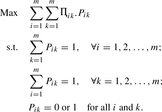
Step 6. Define the permutation matrix P as a square ($m\times m$) matrix and set up the following linear assignment model according to the  value. The linear assignment model can be written in the following linear programming format:
 Step 7. Solve the linear assignment model, and obtain the optimal permutation matrix ${P^{\ast }}$ for all i and k.
Table 6
Weightedrank frequency matrix  .
.
| Alternatives | 1st | 2nd | $\cdots \hspace{0.1667em}$ | mth |
| ${A_{1}}$ | $\cdots \hspace{0.1667em}$ | |||
| ${A_{2}}$ | $\cdots \hspace{0.1667em}$ | |||
| ⋮ | ⋮ | ⋮ | ⋱ | ⋮ |
| ${A_{m}}$ | $\cdots \hspace{0.1667em}$ |
Step 8. Calculate the internal multiplication of matrix ${P^{\ast }}.A={P^{\ast }}.\left[\begin{array}{c}{A_{1}}\\ {} {A_{2}}\\ {} \vdots \\ {} {A_{m}}\end{array}\right]$ and obtain the optimal order of alternatives.
The proposed algorithm has the following advantages. First, evaluation values are given as spherical fuzzy sets, which can consider the indeterminacy degree of decision-makers’ comments about alternatives. Second, the linear assignment method has been used to rank alternatives to avoid the effect of subjectivity.
4 An Application to Wind Power Farm Location Selection
In this section, a numerical example adapted from Kutlu Gündoğdu and Kahraman (2019b) illustrates the feasibility and practical advantages of the newly proposed method. This problem aims to select the best site location in order to establish wind power farms. The most preferred four cities (A1: Canakkale, A2: Manisa, A3: Izmir and A4: Balıkesir) are evaluated as alternatives. Four criteria have been determined in order to evaluate these alternatives. Criteria are environmental conditions (C1), economical situations (C2), technological opportunities (C3), and site characteristics (C4). The weights of alternatives obtained from the pairwise comparison matrix are $w=(0.360,0.158,0.169,0.313)$ for each criterion, respectively. Three decision-makers are going to evaluate the above four possible alternatives according to four criteria based on spherical linguistic terms, as presented in Table 1. The proposed method is used to rank alternatives.
Step 1. Construct the spherical fuzzy decision matrix based on evaluations of three decision-makers. The decision matrices are presented in Tables 7, 8, and 9.
Table 7
Decision matrix based on comments of ${\textbf{\mathit{DM}}_{\mathbf{1}}}$.
| Alternatives | ${C_{1}}$ | ${C_{2}}$ | ${C_{3}}$ | ${C_{4}}$ |
| ${A_{1}}$ | $(0.6,0.4,0.3)$ | $(0.5,0.4,0.4)$ | $(0.3,0.7,0.2)$ | $(0.5,0.4,0.4)$ |
| ${A_{2}}$ | $(0.5,0.4,0.4)$ | $(0.3,0.7,0.2)$ | $(0.3,0.7,0.2)$ | $(0.4,0.6,0.3)$ |
| ${A_{3}}$ | $(0.6,0.4,0.3)$ | $(0.2,0.8,0.1)$ | $(0.5,0.4,0.4)$ | $(0.5,0.4,0.4)$ |
| ${A_{4}}$ | $(0.7,0.3,0.2)$ | $(0.4,0.6,0.3)$ | $(0.5,0.4,0.4)$ | $(0.7,0.3,0.2)$ |
Table 8
Decision matrix based on comments of ${\textbf{\mathit{DM}}_{\mathbf{2}}}$.
| Alternatives | ${C_{1}}$ | ${C_{2}}$ | ${C_{3}}$ | ${C_{4}}$ |
| ${A_{1}}$ | $(0.5,0.4,0.4)$ | $(0.7,0.3,0.2)$ | $(0.3,0.7,0.2)$ | $(0.6,0.4,0.3)$ |
| ${A_{2}}$ | $(0.4,0.6,0.3)$ | $(0.5,0.4,0.4)$ | $(0.3,0.7,0.2)$ | $(0.5,0.4,0.4)$ |
| ${A_{3}}$ | $(0.6,0.4,0.3)$ | $(0.3,0.7,0.2)$ | $(0.6,0.4,0.3)$ | $(0.5,0.4,0.4)$ |
| ${A_{4}}$ | $(0.5,0.4,0.4)$ | $(0.4,0.6,0.3)$ | $(0.4,0.6,0.3)$ | $(0.8,0.2,0.1)$ |
Step 2. Aggregate the decision matrices using Eq. (15) into a single decision matrix, as given in Table 10.
Table 9
Decision matrix based on comments of ${\textbf{\mathit{DM}}_{\mathbf{3}}}$.
| Alternatives | ${C_{1}}$ | ${C_{2}}$ | ${C_{3}}$ | ${C_{4}}$ |
| ${A_{1}}$ | $(0.7,0.3,0.2)$ | $(0.6,0.4,0.3)$ | $(0.5,0.4,0.4)$ | $(0.5,0.4,0.4)$ |
| ${A_{2}}$ | $(0.5,0.4,0.4)$ | $(0.4,0.6,0.3)$ | $(0.4,0.6,0.3)$ | $(0.6,0.4,0.3)$ |
| ${A_{3}}$ | $(0.6,0.4,0.3)$ | $(0.3,0.7,0.2)$ | $(0.7,0.3,0.2)$ | $(0.5,0.4,0.4)$ |
| ${A_{4}}$ | $(0.7,0.3,0.2)$ | $(0.7,0.3,0.2)$ | $(0.7,0.3,0.2)$ | $(0.9,0.1,0.0)$ |
Step 3. Calculate each alternative’s score value based on each criterion using Eq. (13). The results are shown in Table 11.
Table 10
Aggregated decision matrix.
| Alternatives | ${C_{1}}$ | ${C_{2}}$ | ${C_{3}}$ | ${C_{4}}$ |
| ${A_{1}}$ | $(0.61,0.37,0.30)$ | $(0.61,0.37,0.30)$ | $(0.38,0.58,0.30)$ | $(0.53,0.40,0.37)$ |
| ${A_{2}}$ | $(0.47,0.46,0.37)$ | $(0.41,0.56,0.32)$ | $(0.34,0.67,0.24)$ | $(0.51,0.46,0.34)$ |
| ${A_{3}}$ | $(0.60,0.40,0.30)$ | $(0.27,0.73,0.17)$ | $(0.61,0.37,0.30)$ | $(0.50,0.40,0.40)$ |
| ${A_{4}}$ | $(0.65,0.33,0.27)$ | $(0.54,0.48,0.26)$ | $(0.56,0.42,0.30)$ | $(0.82,0.18,0.11)$ |
Step 4. Establish the rank frequency matrix based on the scored value matrix. First, we have to determine each alternative’s ranking based on each criterion, as shown in Table 12. Then, the rank frequency matrix λ is established as in Table 13. For example, observe that $A1$ has the first rank once (on ${C_{2}}$), the second rank twice (on ${C_{1}}$ and ${C_{4}}$), the third rank once (on ${C_{3}}$) and none fourth rank. Thus, ${\lambda _{11}}=1$, ${\lambda _{12}}=2$, ${\lambda _{13}}=1$ and ${\lambda _{14}}=0$.
Table 11
The score value of each alternative.
| Alternatives | ${C_{1}}$ | ${C_{2}}$ | ${C_{3}}$ | ${C_{4}}$ |
| ${A_{1}}$ | 0.16 | 0.16 | 0.05 | 0.08 |
| ${A_{2}}$ | 0.02 | 0.02 | 0.02 | 0.03 |
| ${A_{3}}$ | 0.14 | 0.00 | 0.16 | 0.05 |
| ${A_{4}}$ | 0.22 | 0.06 | 0.09 | 0.57 |
Table 12
Rankingof each alternative based on each criterion.
| Ranking | ${C_{1}}$ | ${C_{2}}$ | ${C_{3}}$ | ${C_{4}}$ |
| 1st | $A4$ | $A1$ | $A3$ | $A4$ |
| 2nd | $A1$ | $A4$ | $A4$ | $A1$ |
| 3rd | $A3$ | $A2$ | $A1$ | $A2$ |
| 4th | $A2$ | $A3$ | $A2$ | $A3$ |
Step 5. Compute  and further establish the weighted rank frequency matrix
  , as shown in Table 14. For example, consider
  in the following:

Table 13
Rank frequency matrix λ.
| Alternatives | 1st | 2nd | 3rd | 4th |
| $A1$ | 1 | 2 | 1 | 0 |
| $A2$ | 0 | 0 | 2 | 2 |
| $A3$ | 1 | 0 | 1 | 2 |
| $A4$ | 2 | 2 | 0 | 0 |
Step 6. Construct the linear assignment model as follows. This binary mathematical model’s objective function tries to maximize the sum of the weights of alternatives by choosing the optimal order.
\[\begin{aligned}{}& \operatorname{Max}Z=0.158{P_{11}}+0.673{P_{12}}+0.169{P_{13}}+0.471{P_{23}}+0.529{P_{24}}+0.169{P_{31}}\\ {} & \phantom{\operatorname{Max}Z=}+0.36{P_{33}}+0.471{P_{34}}+0.673{P_{41}}+0.327{P_{42}}\\ {} & \text{s.t.}\\ {} & \hspace{1em}{P_{11}}+{P_{12}}+{P_{13}}+{P_{14}}=1,\\ {} & \hspace{1em}{P_{21}}+{P_{22}}+{P_{23}}+{P_{24}}=1,\\ {} & \hspace{1em}{P_{31}}+{P_{32}}+{P_{33}}+{P_{34}}=1,\\ {} & \hspace{1em}{P_{41}}+{P_{42}}+{P_{43}}+{P_{44}}=1,\\ {} & \hspace{1em}{P_{11}}+{P_{21}}+{P_{31}}+{P_{41}}=1,\\ {} & \hspace{1em}{P_{12}}+{P_{22}}+{P_{32}}+{P_{42}}=1,\\ {} & \hspace{1em}{P_{13}}+{P_{23}}+{P_{33}}+{P_{43}}=1,\\ {} & \hspace{1em}{P_{14}}+{P_{24}}+{P_{34}}+{P_{44}}=1,\\ {} & \hspace{1em}{P_{ik}}=0\hspace{2.5pt}\text{or}\hspace{2.5pt}1\hspace{1em}\text{for}\hspace{2.5pt}i=1,2,3,4;\hspace{2.5pt}k=1,2,3,4.\end{aligned}\]
Table 14
Weighted rank frequency matrix  .
.
| Alternatives | 1st | 2nd | 3rd | 4th |
| $A1$ | 0.158 | 0.673 | 0.169 | 0 |
| $A2$ | 0 | 0 | 0.471 | 0.529 |
| $A3$ | 0.169 | 0 | 0.36 | 0.471 |
| $A4$ | 0.673 | 0.327 | 0 | 0 |
Step 7. Solve the above mathematical model by using GAMS 24.1.3 software, and the results are obtained as follows:
 After solving the model, the results are ${P_{12}}=1$, ${P_{23}}=1$, ${P_{34}}=1$ and ${P_{41}}=1$. Also, the objective function of the assignment model is $z=2.288$.
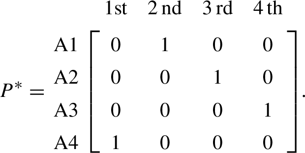
Step 8. Apply the permutation matrix ${P^{\ast }}$ to the matrix of alternatives (A) to obtain the optimal order of alternatives.
\[ A\times {P^{\ast }}=({A_{1}},{A_{2}},{A_{3}},{A_{4}})\times \left[\begin{array}{c@{\hskip4.0pt}c@{\hskip4.0pt}c@{\hskip4.0pt}c}0\hspace{1em}& 1\hspace{1em}& 0\hspace{1em}& 0\\ {} 0\hspace{1em}& 0\hspace{1em}& 1\hspace{1em}& 0\\ {} 0\hspace{1em}& 0\hspace{1em}& 0\hspace{1em}& 1\\ {} 1\hspace{1em}& 0\hspace{1em}& 0\hspace{1em}& 0\end{array}\right]=({A_{4}},{A_{1}},{A_{2}},{A_{3}}).\]
The optimal ranking order of the four alternatives is ${A_{4}}>{A_{1}}>{A_{2}}>{A_{3}}$. Thus, the best alternative is ${A_{4}}$. When we compared the results with Kutlu Gündoğdu and Kahraman (2019b) and Gündoğdu and Kahraman (2019b) researches, the ordering of the alternatives is slightly different. However, the best alternative is the same and ${A_{4}}$ in all approaches. The comparison between the proposed approach and spherical fuzzy AHP and spherical fuzzy WASPAS methods is given in Table 15. The suggested method has several advantages. The first advantage is that the method reduces decision-makers’ subjectivity, which directly calculates the relative closeness of every alternative to the ideal solution. The second is that the linear assignment method provides a general preference ranking of the alternatives based on a set of criterion-wise rankings.5 Conclusion
In recent years, spherical fuzzy sets have been very widespread in almost all branches. Spherical fuzzy sets are the last extension of the ordinary fuzzy sets that should satisfy the condition that the squared sum of membership degree and non-membership degree, and hesitancy degree must be equal to or less than one. In this study, the classical linear assignment model is extended to the spherical fuzzy linear assignment model, and the developed method is applied to site selection of wind power farm problem. In the proposed SF-LAM method, we firstly get the weight vector of the criteria using the pairwise comparison matrix. Then, the linear assignment method is performed to get the optimal preference ranking of the alternatives according to a set of criteria-wise rankings within the context of SFS. It has been successfully solved by SF-LAM and compared with SF-AHP and SF-WASPAS methods for the same problem. The ranking results in both methods are different, but the best alternative is the same in both approaches. The judgments of multi-DMs can be incorporated into the proposed method. Using the linear assignment model, we can determine the optimal ranking of the alternatives.
As the limitation of the proposed method, a single-objective mathematical model that just considers the maximization of criteria weights is used together with subjective linguistic judgments. To cope with these limitations, we suggest employing a multi-objective model to consider other influencing factors for further research. The weights of criteria could also be obtained using different methods such as maximizing deviation method. Another further research may be the usage of Pythagorean fuzzy sets in the proposed method instead of spherical fuzzy sets for comparative purposes.


 .
. .
.