1 Introduction
A secret sharing scheme is any method of distributing a secret amongst a number of participants in such a way that any authorized group of participants can recover the secret, while unauthorized sets of participants are unable to obtain any information about the secret using their shares. In a k-out-of-n secret sharing scheme, there are n participants and every collection of k or more participants is authorized to recover the secret, while fewer than k participants constitute an unauthorized set. The number k is referred to as the threshold and the scheme is usually referred to as a $(k,n)$-threshold secret sharing scheme, or a $(k,n)$-scheme for short. While there exist other approaches such as those where authorized sets of participants are specified by properties other than merely the size of the subset, in this work we focus on $(k,n)$-schemes.
The concept of secret sharing was introduced in 1979 independently by Shamir (
1979) and Blakley
et al. (
1979). Shamir’s method is based on polynomial interpolation in the field
${\mathbb{F}_{p}}$ of integers modulo
p, whereas Blakley’s method is based on hyperplane geometry. In the early eighties, Mignotte (
1982) and Asmuth and Bloom (
1983) proposed a threshold secret sharing approach based on the Chinese remainder theorem. Secret sharing schemes are important primitives in a number of cryptographic applications such as threshold signature (authentication) schemes (Desmedt and Frankel,
1991), access control (Naor and Wool,
1998), electronic voting (Schoenmakers,
1999), distributed storage systems (Wylie
et al.,
2000), etc.
Because of the widespread use of digital images, development of secret image sharing schemes (SIS) where the secret is a digital image have attracted the attention of researchers. In the context of an SIS, shares are often referred to as shadow images. We refer to a
$(k,n)$-threshold secret image sharing scheme as a
$(k,n)$-SIS for short. There are challenges specific to secret image sharing. For example, secret sharing was originally introduced for sharing cryptographic keys, thus sizes of shares were not much of a concern. On the other hand, since digital images are typically large, one is concerned with how large each shadow image is in comparison to the original secret. While Shamir’s scheme produces shares of the same size as the secret itself, Thien and Lin (
2002) proposed a
$(k,n)$-SIS inspired by Shamir’s scheme whose shadow images are of size
$1/k$ the size of the secret. Lin and Tsai (
2004) extended Shamir’s scheme in proposing a secret image sharing scheme with the capabilities of steganography and authentication. Chang
et al. (
2008) showed that this scheme suffers from weak authentication and low quality of stego-images. In Bai (
2006), Bai proposed a
$(k,n)$-SIS based on matrix projection in conjunction with Thien and Lin’s approach (Thien and Lin,
2002). del Rey (
2008) proposed a
$(2,n)$-SIS using binary matrices. Rey’s scheme is shown to suffer from some drawbacks if the matrices are not of low enough rank (Elsheh and Hamza,
2010). Many Shamir-based SIS use arithmetic in the fields
${\mathbb{F}_{251}}$ or
${\mathbb{F}_{257}}$ to accommodate 8-bit intensity values of digital images. This choice renders such schemes lossy since they involve truncation of some values. Hu
et al. (
2012) proposed a lossless
$(k,n)$-SIS over the Galois field
${\mathbb{F}_{{2^{8}}}}$. In El-Latif
et al. (
2013), Abd El-Latif
et al. proposed a secret image sharing scheme based on random grids and error diffusion and a chaotic cat map for the generation of meaningful shadow images. Wu (
2013) proposed a variant of Thien–Lin’s scheme (Thien and Lin,
2002) which uses prime number 257 as a replacement for 251 in Thien–Lin’s approach. Wu’s scheme has a low distortion rate, and is more applicable for light images (Wu,
2013). However, due the overflow caused in the generation phase of this scheme, reconstruction of the secret image is more computationally intensive than in the case of Thien–Lin’s scheme. In Zarepour-Ahmadabadi
et al. (
2016), Zarepour-Ahmadabadi
et al. proposed an SIS based on cellular automata. Deng
et al. (
2017) proposed a
$(2,n)$-threshold SIS based on basic vector operations and coherence superposition. Kanso and Ghebleh (
2017) proposed a variant of Thien and Lin’s scheme based on cyclic shifting to improve the quality of the reconstructed secret image. Kabirirad and Eslami (
2018) proposed a multi secret SIS based on Boolean operations whose drawback is that each generated shadow image has the same size as the secret image. Ghebleh and Kanso (
2018) proposed a
$(k,n)$-SIS based on Shamir’s approach and arithmetic in a field
${\mathbb{F}_{p}}$ where
p is a large prime, to facilitate the use of (concatenated) multiple intensity values of the secret image as a single coefficient. While still lossy, this method enhances the quality of the reconstructed secret. Ding
et al. (
2018) proposed a scheme based on matrix theory and Shamir’s construction. Recently, Kanso and Ghebleh (
2018) proposed a
$(k,n)$-threshold secret sharing scheme for medical images based on Shamir’s approach and the high redundancy in medical images. Some secret image sharing schemes such as Chang and Hwang (
1998), Chang
et al. (
2006), Chen
et al. (
2009), Le
et al. (
2011) employ vector quantization (VQ) methods (Gray,
1984; Gersho and Gray,
2012; Simić
et al.,
2018) to compress the secret image, which results in further reduction in the sizes of the shadow images.
A majority of existing secret image sharing schemes in the literature are based on one of Shamir’s (
1979), Blakley’s
et al., (
1979), Mignotte’s, (
1982) and Asmuth and Bloom’s, (
1983) approaches. Furthermore, many of the existing schemes are lossy and restore the secret image with some distortion which may not be acceptable in certain applications. Moreover, some existing SIS suffer from weak authentication and security issues. The aim of this research is to present a secret sharing scheme that has improved performance over existing work.
In this paper, we propose a lossless linear algebraic $(k,n)$-SIS. As illustrated later, the proposed scheme is a generalization of Shamir’s secret sharing scheme based on polynomial interpolation. The scheme associates a vector ${\mathbf{v}_{i}}$ to the ith participant in the k-dimensional vector space ${\mathbb{F}_{q}^{k}}$ over the Galois field ${\mathbb{F}_{q}}$, where q is a power of 2. The ith share is then computed as a linear combination of the vectors ${\mathbf{v}_{i}}$ with coefficients computed from the secret. For the threshold property of secret sharing, and for security of shares, some admissibility conditions (such as linear independence of certain sets) are enforced on the vectors ${\mathbf{v}_{i}}$. Empirical results presented in the paper illustrate the proposed scheme’s performance. These include security of shadow images and the recovery process. More specifically, it is shown that the produced shadow images satisfy randomness properties which in turn means that the shadow images do not reveal any meaningful information about the secret image. Moreover, shadow images have little or no correlation. It is also shown that any unauthorized collection of shadow images fails to produce any information about the secret image. The proposed scheme is lossless, which means that it can be used for sharing any type of digital data (as secret), including text and binary files such as compressed images generated via vector quantization.
The paper is organized as follows: In Section
2, we present the necessary background and notation. Section
3 provides a detailed description of the proposed scheme. Simulations are presented in Section
4 to showcase the efficiency of the scheme, the properties of the generated shadow images and security analysis. Section
5 presents a comparison of the scheme with existing work. Finally, we end the paper with some concluding remarks.
2 Background and Notation
We propose a secret image sharing scheme based on Shamir’s approach (Shamir,
1979). In this section we lay out the necessary background and notation, as well as differences between the proposed scheme and Shamir’s scheme.
Shamir’s
$(k,n)$-scheme is based on polynomial interpolation in the field
${\mathbb{F}_{p}}$ where
p is a prime number. To share secret
$D\in \{0,1,\dots ,p-1\}$, a polynomial
is chosen at random with
${a_{0}}=D$. Then the values
$f(i)$ where
$i\in \{1,2,\dots ,n\}$ are computed and distributed to the participants as shares. With the obvious conditions that
$k\leqslant n<p$, the polynomial interpolation theorem guarantees that every
k shares suffice to recover
$f(x)$, and in particular the secret
D. Following the notation of Spiez
et al. (
2009), Schinzel
et al. (
2010), this can be generalized by fixing pairwise distinct nonzero values
${x_{1}},{x_{2}},\dots ,{x_{n}}\in {\mathbb{F}_{p}}$ and using
${y_{i}}=f({x_{i}})$ as the
ith share. With this notation, computation of shares can be summarized as
Let
$\mathbf{a}=({a_{0}},{a_{1}},\dots ,{a_{k-1}})$,
$\mathbf{y}=({y_{1}},{y_{2}},\dots ,{y_{n}})$, and
X be the
$n\times k$ matrix in the above equation. For convenience, we identify vectors such as
a and
y with their row or column matrix representation. Then the above equation can be written as
Simple linear algebra gives the following:
-
• For guaranteed recovery of the secret
${a_{0}}$ from any
k shares, all
$k\times k$ submatrices of
X must be nonsingular. While in the field of real numbers this condition is satisfied by the assumption that the components of the track
$\mathbf{x}=({x_{1}},{x_{2}},\dots ,{x_{n}})$ are positive and pairwise distinct, in a finite field
$\mathbb{F}$ this is not necessarily the case. For example, the matrices
are singular over
${\mathbb{F}_{7}}$.
-
• If a $(k-1)\times (k-1)$ submatrix of X induced by the rows $2,3,\dots ,k$ and columns ${j_{1}},{j_{2}},\dots ,{j_{k-1}}$ is singular, then the $k-1$ shares ${y_{{j_{1}}}},{y_{{j_{2}}}},\dots ,{y_{{j_{k-1}}}}$ suffice to recover the secret ${a_{0}}$. Thus for the threshold property of the secret sharing scheme to be satisfied, we need all such $(k-1)\times (k-1)$ submatrices of X to be nonsingular.
The track
$\mathbf{x}=({x_{1}},{x_{2}},\dots ,{x_{n}})$ is said to be admissible if it satisfies the nonsingularity conditions discussed above. Admissible tracks are studied in Schinzel
et al. (
2010), Spież
et al. (
2012).
In this work, we consider a general matrix X for computation of the shares vector y. By destroying the algebraic relations between columns of X, this idea allows more “randomness” in the shares, thus potentially making the scheme more secure. On the other hand, the lack of algebraic relations in X renders the theoretical study admissibility impractical, and each X must be verified directly. We propose to choose X randomly from the set of all $n\times k$ matrices over the given field, then check its admissibility. If the field has large enough cardinality, this process has a high probability of success.
Thien and Lin (
2002) proposed a secret image sharing scheme (SIS) where all coefficients of the polynomial
$f(x)$, namely components of
a, are chosen from the secret. As long as the secret image is properly shuffled to eliminate correlations between entries of
a, this scheme works similarly to Shamir’s scheme with the following two advantages:
-
• While in Shamir’s scheme each share has the same size as the secret, shares of Thien and Lin’s scheme have size $1/k$ of the size of the secret.
-
• A singular $(k-1)\times (k-1)$ submatrix of X would compromise the threshold property only for one coefficient ${a_{i}}$ which is only part of the secret. So while admissibility of X must be checked, if it is overlooked, it does not necessarily compromise the whole secret.
We follow the same approach in this work and pick all components of the vector
a from the shuffled secret image. Since a digital image typically has a large size compared to the parameters
k and
n of the scheme, elements of the secret are processed
k at a time. This can be utilized by allowing
y and
a to have more than one column. More specifically, we write the proposed SIS as
where
S is a
$k\times m$ matrix obtained by padding, shuffling, and reshaping the secret image,
X is an admissible
$n\times k$ transformation matrix, and the
$n\times m$ matrix
Y is the matrix of shares, whose
ith row constitutes the
ith share.
The final difference between the proposed scheme, Shamir’s, and Thien and Lin’s schemes is the use of the field ${\mathbb{F}_{q}}$ where $q={2^{\alpha }}$ instead of ${\mathbb{F}_{p}}$ where p is a prime. Since digital media typically contain values from a domain $\{0,1,\dots ,{2^{\alpha }}-1\}$, the use of a field ${\mathbb{F}_{p}}$ involves truncation of some values which renders such secret sharing schemes lossy. Depending on the application, this might be acceptable or not. While computations in ${\mathbb{F}_{p}}$ are faster, the field ${\mathbb{F}_{q}}$ where $q={2^{\alpha }}$ is the natural choice for a lossless scheme. Since digital images typically consist of bytes of information, it is convenient for α to be a multiple of 8. If $\alpha =8\beta $, the entries ${s_{ij}}$ of the matrix S are each a concatenation of β entries of the secret image.
It should be noted that as mentioned above, for the random selection of the transformation matrix X to have a high probability of admissibility, the field ${\mathbb{F}_{q}}$ must have a large cardinality. In the empirical analysis presented in this work we choose $\alpha =16$ and carry all computations in the field ${\mathbb{F}_{q}}$ where $q={2^{16}}$.
3 The Proposed Scheme
Following the notation of the previous section, the proposed SIS is summarized as
where
X is an admissible transformation matrix,
S is the secret image (subjected to concatenation of entries, shuffling, padding and reshaping), and
Y is the shares matrix. All these matrices have entries from a field
${\mathbb{F}_{q}}$ where
$q={2^{\alpha }}={2^{8\beta }}$ for some chosen parameter
β. In this section, we present in more detail the generation of the matrices
X and
S, and the generation of shadow images using them. For added security, the secret image may be divided into several blocks, where each block is processed separately (with an independent transformation matrix
X). In this case a parameter
m specified by the user defines the number of columns of the matrix
S corresponding to each block.
The parameters of the proposed scheme which are kept constant throughout this section are the number
β of bytes in each entry of
S, the number
n of the participants, the threshold
k, and the block size
m. With fixed
β, we also fix an ordering of the elements of the field
${\mathbb{F}_{q}}$ where
$q={2^{8\beta }}$, say
${\mathbb{F}_{q}}=\{{f_{0}},{f_{1}},{f_{2}},\dots ,{f_{q-1}}\}$ where
${f_{0}}=0$. Throughout our discussions, we use the correspondence
to move between the field
${\mathbb{F}_{q}}$ and the group
${\mathbb{Z}_{q}}$ of integers modulo
q.
3.1 The Cat Map
Arnold’s cat map (Arnol’d and Avez,
1968; Rong and Xiaoning,
1998) is a chaotic map studied extensively in the literature. It is known to generate pseudo-random numbers which are essential in cryptographic applications (Chen
et al.,
2004; Kanso and Ghebleh,
2012,
2013,
2015). Chen
et al. (
2004) proposed a 3-dimensional generalization of the cat map defined by
where
${\mathbf{x}_{i}}$ is the state vector of the map whose entries are in the interval
$[0,1)$, and
is defined using positive integer parameters
${a_{x}}$,
${a_{y}}$,
${a_{z}}$,
${b_{x}}$,
${b_{y}}$,
${b_{z}}$. It is known (Chen
et al.,
2004; Kanso and Ghebleh,
2012) that iterated applications of this map generate a pseudo-random sequence of values in the interval
$[0,1)$ by taking components of the state vector.
3.2 Generation of the Transformation Matrix X
An admissible transformation matrix must be generated for each block of the secret. To avoid unnecessary complications, we refrain from including a block index in the notation and refer to this matrix simply as X. Let ${\mathbf{v}_{i}}$ denote the ith row of X where $1\leqslant i\leqslant n$. For X to be admissible, the following conditions must be satisfied:
The condition (A1) means that every
k of the vectors
${\mathbf{v}_{1}},\dots ,{\mathbf{v}_{n}}$ must be linearly independent in the vector space
${\mathbb{F}_{q}^{k}}$. One would imagine that for this condition to be satisfied,
n cannot be too large. On the other hand, provided that
${\mathbb{F}_{q}}$ has large enough cardinality, this does not pose a practical restrain on the proposed scheme. Indeed it is known (Maneri and Silverman,
1966) that the maximum number of such vectors (the maximum possible choice of
n) is at least
$|{\mathbb{F}_{q}}|+1={2^{8\beta }}+1$ which is much larger than practical requirements of an SIS.
Algorithm 1
Generation of a transformation matrix
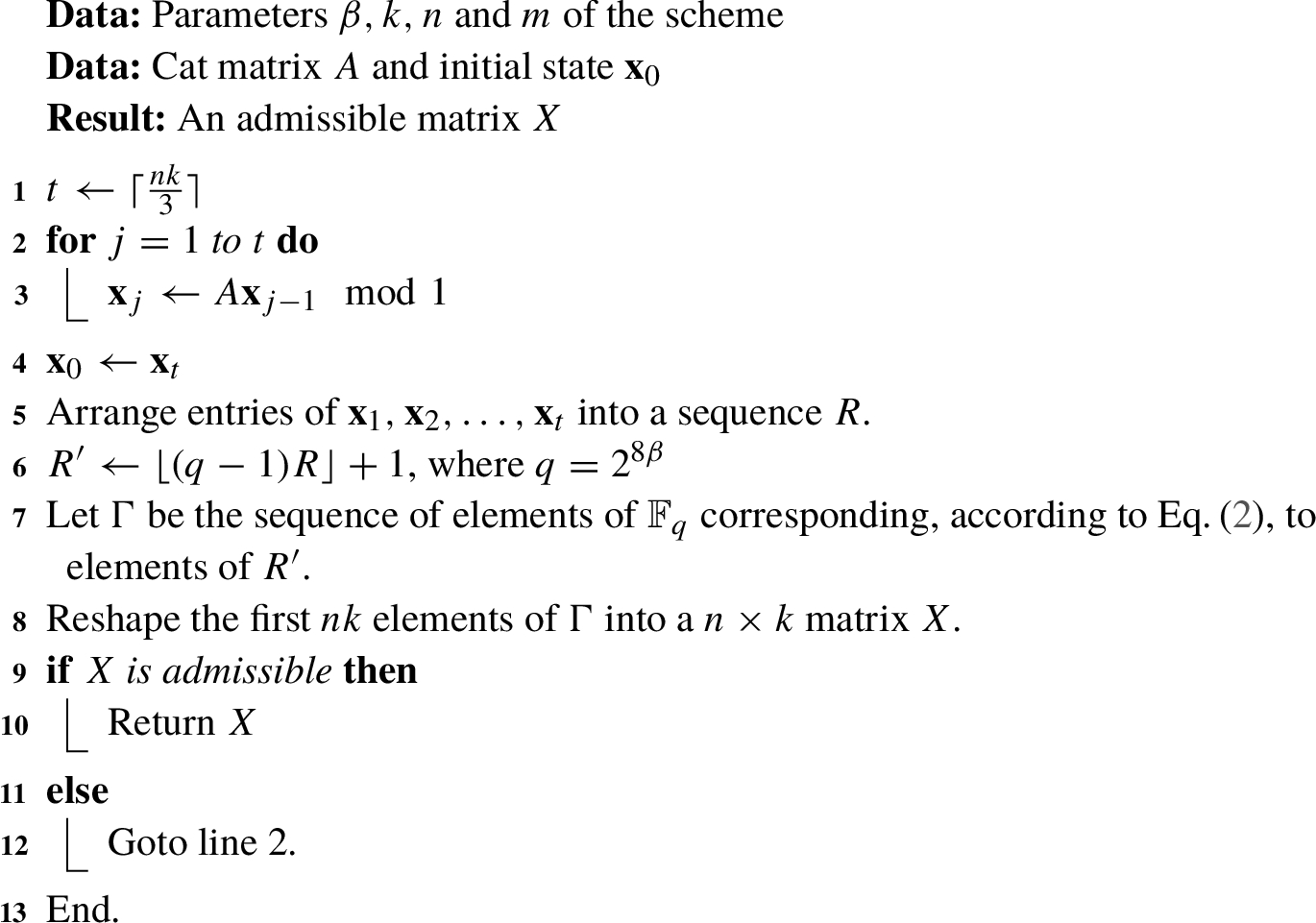
Our approach for generation of an admissible transformation matrix
X, as described in Algorithm
1, is to populate a
$n\times k$ matrix by randomly chosen nonzero elements of
${\mathbb{F}_{q}}$, then to test whether this matrix is admissible. If not, the matrix at hand is simply discarded and a new one is generated. The simple structure of the cat map used to generate pseudo-random numbers accommodates fast generation of these matrices. On the other hand, testing admissibility is more computation-intensive since it involves verifying non-singularity of all
$k\times k$ and
$(k-1)\times (k-1)$ submatrices. Our experimental results presented in Table
1, with
$\beta =2$ and small values of
k and
n, show that with high probability, the first generated matrix is indeed admissible.
Table 1
The ratio of admissible matrices X out of 10000 randomly generated $n\times k$ matrices.
| n |
k |
| 2 |
3 |
4 |
5 |
6 |
| 2 |
0.9999 |
– |
– |
– |
– |
| 3 |
0.9996 |
0.9997 |
– |
– |
– |
| 4 |
1.0000 |
0.9998 |
0.9999 |
– |
– |
| 5 |
1.0000 |
0.9989 |
0.9994 |
0.9996 |
– |
| 6 |
0.9997 |
0.9991 |
0.9987 |
0.9988 |
0.9992 |
3.3 Generation of the Matrix S
The matrix
S of Eq. (
1) is generated from the plain secret image
P. Since
S is of size
$k\times m$, it contains
$b=mk\beta $ bytes of
P. We assume
P is padded in preprocessing so that its size in bytes is a multiple of
b. The plain secret image
P is also shuffled in preprocessing. The shuffling is performed according to the outputs of the cat map as follows. A pseudo-random sequence
R of length
$|P|$ is generated similarly to lines 1–5 of Algorithm
1 with initial state
${\mathbf{x}^{\prime }_{0}}$, then a permutation
π is found which sorts
R. The shuffled image
Q is obtained by applying the permutation
π on
P.
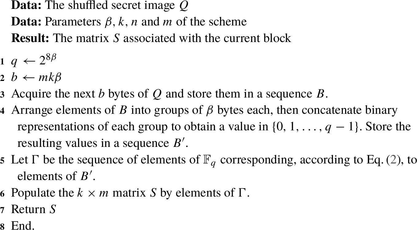
For each block, a matrix
S is generated using the next
b bytes of
Q. Algorithm
2 presents details of this process. Again we refrain from indicating a block index in the naming of variables such as
S to avoid cumbersome notation.
Algorithm 2
Generation of the matrix S
3.4 Generation of Shadow Images
For each block, with the matrices
X and
S in hand, the share matrix
Y can be computed according to Eq. (
1). For each
$1\leqslant i\leqslant n$, the
ith row of the resulting matrix
Y constitutes a block of the
ith share. The
ith shadow image is generated from the collection of all such rows by converting each element to an integer via the correspondence of Eq. (
2), then breaking each integer value to
β bytes. For added security we shuffle the
ith shadow image according to a pseudo-random sequence
${R^{(i)}}$ of length
$\frac{1}{k}|P|$ generated similarly to lines 1–5 of Algorithm
1 with initial state
${\mathbf{x}_{0}^{(i)}}$. Let
${\pi ^{(i)}}$ denote the permutation which sorts
${R^{(i)}}$. We denote the shuffled shadow image that is obtained by applying
${\pi ^{(i)}}$ to the
ith shadow image by
${H_{i}}$. The share (shadow image)
${H_{i}}$ may be reshaped to a rectangular array for presentation as an image.
3.5 Secret Key
The secret key of the proposed scheme consists of the parameters ${a_{x}}$, ${a_{y}}$, ${a_{z}}$, ${b_{x}}$, ${b_{y}}$, ${b_{z}}$ of the cat matrix, as well as the initial states ${\mathbf{x}_{0}}$, ${\mathbf{x}^{\prime }_{0}}$ and ${\mathbf{x}_{0}^{(i)}}$, where $1\leqslant i\leqslant n$. It should be noted that for added security, different cat matrices may be used for the preprocessing (shuffling) and the transformation matrices.
3.6 Recovery of the Secret Image
We assume that the secret key of the scheme is held at a central authority and is released upon the presentation of shadow images by any authorized set of participants. Suppose that
k shadow images
${H_{{i_{1}}}},{H_{{i_{2}}}},\dots ,{H_{{i_{k}}}}$ are presented to the central authority. The recovery of the secret image is carried out as follows.
-
• Apply the inverse of the shuffling permutation ${\pi ^{({i_{j}})}}$ on each shadow image ${H_{{i_{j}}}}$, for $1\leqslant j\leqslant k$.
-
• Each shadow image is converted to a sequence of elements of
${\mathbb{F}_{q}}$ by grouping every
β bytes into a single integer, and via the correspondence in Eq. (
2). The resulting sequences are then broken-up into blocks, using which a
$k\times m$ submatrix
$\tilde{Y}$ of the matrix
Y associated with each block are obtained. More specifically, each
$\tilde{Y}$ consists of the rows
${i_{1}},{i_{2}},\dots ,{i_{k}}$ of the corresponding matrix
Y.
-
• Using the secret key, the matrix X associated with each block is constructed. We then let $\tilde{X}$ be the $k\times k$ submatrix of X induced by the rows ${i_{1}},{i_{2}},\dots ,{i_{k}}$.
-
• By Eq. (
1), we have
$\tilde{Y}=\tilde{X}S$. On the other hand, by admissibility of
X, the matrix
$\tilde{X}$ is nonsingular. Thus we may compute
$S={(\tilde{X})^{-1}}\tilde{Y}$.
-
• By reversing the transformation of Algorithm
2, the shuffled secret image
Q is reconstructed block by block. The plain secret image
P is now obtained by generating the shuffling permutation
π and applying its inverse on
Q, then removing the padding.
3.7 Delivery of Shares
As outlined above, the secret image can be easily reconstructed upon the presence of the secret key and at least
k shadow images. Therefore, the security of the proposed scheme is compromised if an unauthorized party gets hold of the shares. Therefore, the dealer must securely transmit each shadow image
${H_{i}}$ to its corresponding participant. Depending on the application, this can be accomplished using a secure channel, a cryptographic scheme through a public channel such as one of those proposed in Chen
et al. (
2004), Kanso and Ghebleh (
2012), Fu
et al. (
2018) or a steganographic scheme which hides the presence of shadow images such as one of those proposed in Ghebleh and Kanso (
2014), Fridrich
et al. (
2002).
4 PerformanceAnalysis
In this section, we demonstrate the efficiency of the proposed scheme and its robustness against a number of attacks. The simulation results are based on the following parameters: the number of bytes per value
$\beta =2$, the number of participants
$n=6$, the threshold (minimum number of participants in an authorized set)
$k=4$, and
$m=1024$. For the tests presented in this section, we use the cat matrix
obtained using the parameters
$({a_{x}},{a_{y}},{a_{z}};\hspace{0.1667em}{b_{x}},{b_{y}},{b_{z}})=(2,1,117;\hspace{0.1667em}31,2,3)$.
Recall that each block of the process involves
$mk\beta =8192$ bytes of the secret, resulting in 4096 elements of the field
${\mathbb{F}_{q}}$ with
$q={2^{16}}$. Consider the standard grayscale image Lena of size
$512\times 512$ presented in Fig.
1 to be the secret image. Then each shadow image consists of 65536 bytes since the size of each share is
$1/k$ the size of the secret. For presentation, each
${H_{i}}$ (
$1\leqslant i\leqslant n$) is reshaped into a
$256\times 256$ matrix also denoted by
${H_{i}}$. Figure
2 depicts the six shadow images corresponding to the test image Lena.

Fig. 1
The secret image Lena of size $512\times 512$.
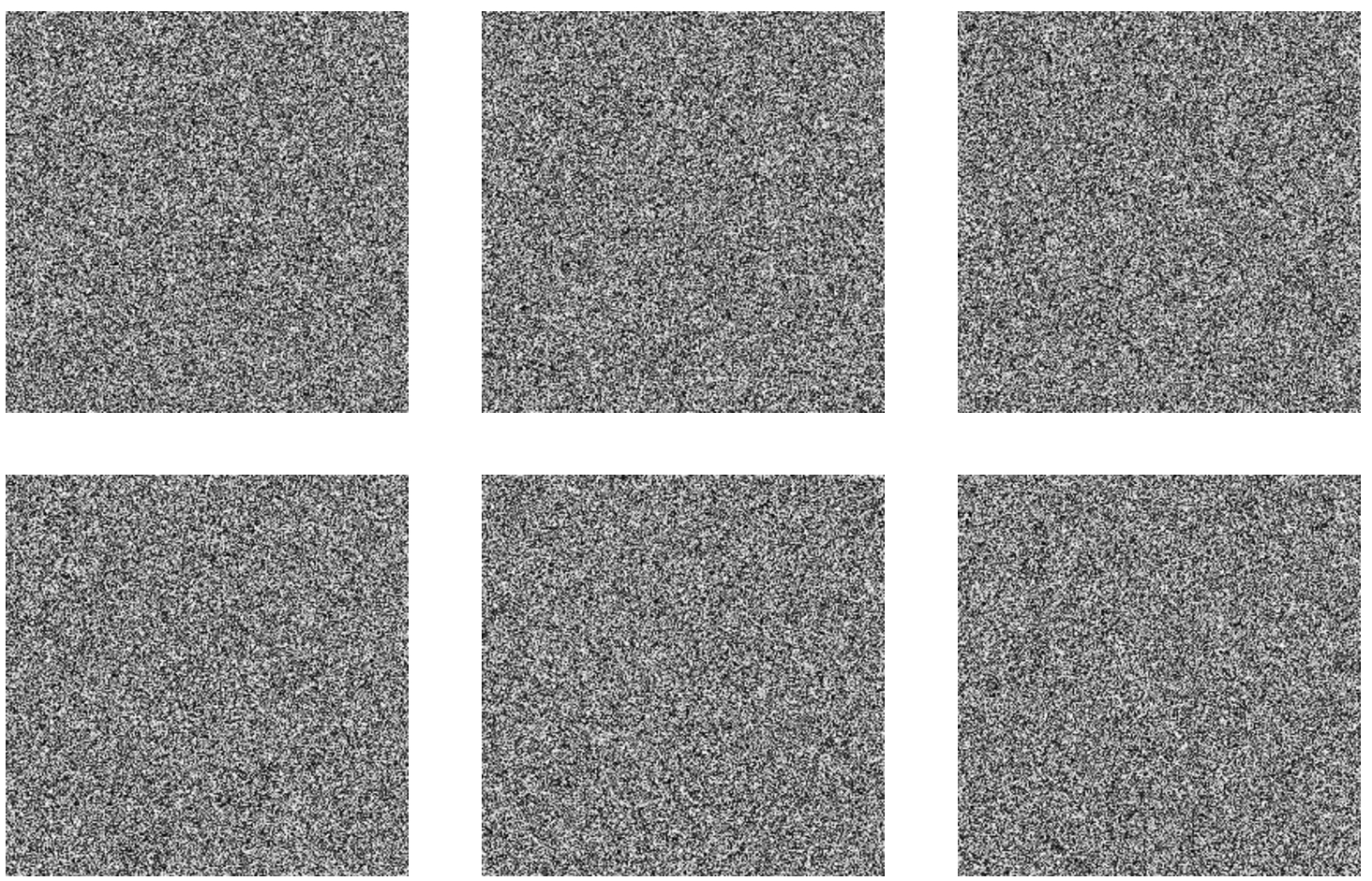
Fig. 2
The shadow images ${H_{1}},{H_{2}},\dots ,{H_{6}}$ corresponding to the test image Lena, where each shadow image has size $256\times 256$.
4.1 Histogram Analysis
The histogram of a given digital image displays the distribution of its tonality. For a meaningful image such as the test Lena image, the histogram shows non-uniform distribution of its tonality, and hence one can derive some information about the content of the image. However, for a truly random image the histogram is almost flat, so no useful information about the image can be derived from it. This test shows that the histogram of each shadow image is almost flat, that is the intensity values are uniformly distributed in
$\{0,1,\dots ,255\}$. Hence, no useful information about the secret can be derived from the shadow images. Figure
3 depicts the histograms of the test image Lena and one sample shadow image from
${H_{1}},{H_{2}},\dots ,{H_{6}}$. The histograms of the other shadow images show similar behaviour.
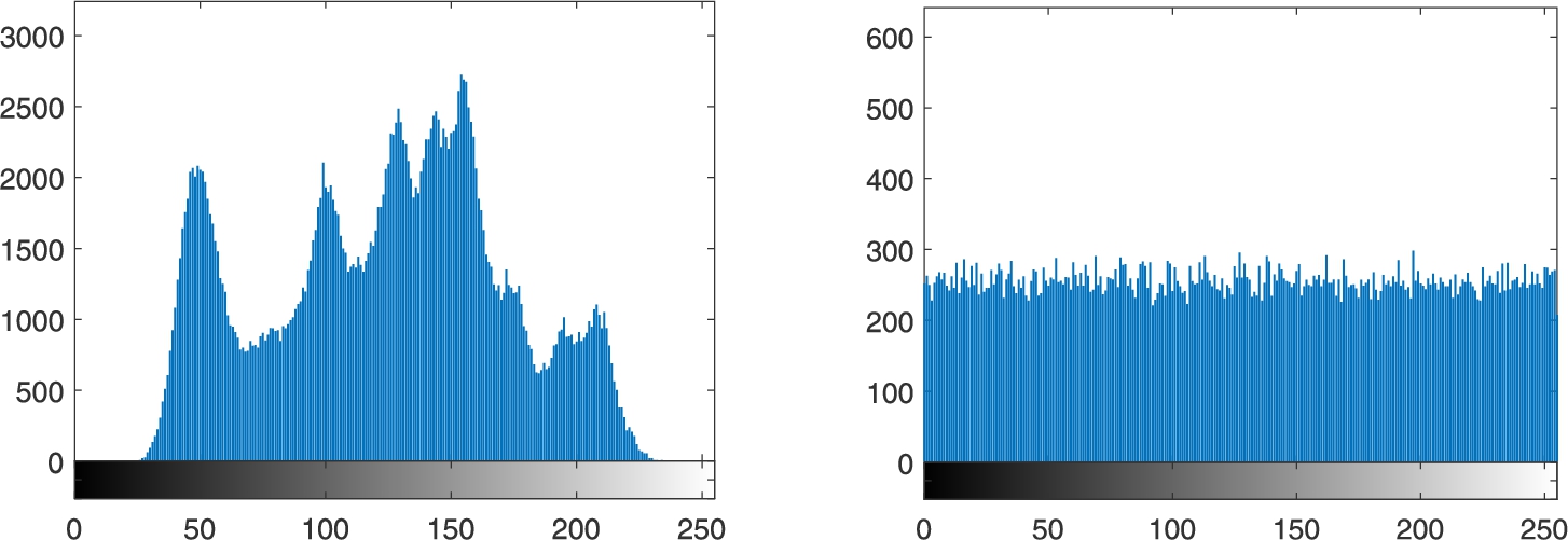
Fig. 3
The histogram of the Lena image (left) and the histogram of a sample shadow image (right).
4.2 Correlation Analysis
Correlation analysis is a randomness test that identifies the strength of relationships between adjacent pixels. Meaningful images such as the test image Lena possess high correlation between adjacent pixels. This test shows that shadow images generated by the proposed scheme have almost no correlation between adjacent pixels.
Consider a sample shadow image, and select
$N=10000$ random pairs of adjacent pixels
${x_{i}}$ and
${y_{i}}$ in the horizontal, vertical and diagonal directions. The correlation coefficient between the two sequences
${\{{x_{t}}\}_{t=1}^{N}}$ and
${\{{y_{t}}\}_{t=1}^{N}}$ is given by
where
${\mu _{x}}$ and
${\mu _{y}}$ denote the mean values of
x and
y, respectively;
${\sigma _{x}}$ and
${\sigma _{y}}$ denote their standard deviations, and
$E[\cdot ]$ is the expected value. The correlation coefficient
${C_{xy}}\in [-1,1]$, where a value 0 indicates no correlation and a value
$\pm 1$ indicates complete correlation between the two sequences.
Table
2 presents the correlation coefficients between
${\{{x_{t}}\}_{t=1}^{N}}$ and
${\{{y_{t}}\}_{t=1}^{N}}$ in (i) the Lena image and (ii) the shadow images. This table shows that the shadow images are almost free of any correlation between adjacent pixels in the horizontal, vertical and diagonal directions.
Table 2
Correlation coefficients of adjacent pixels in the Lena image and its corresponding shadow images.
| Image |
Lena |
${H_{1}}$ |
${H_{2}}$ |
${H_{3}}$ |
${H_{4}}$ |
${H_{5}}$ |
${H_{6}}$ |
| Horizontal |
0.972726 |
0.005061 |
$-0.000394$ |
$-0.002141$ |
0.006671 |
0.020705 |
$-0.013311$ |
| Vertical |
0.985929 |
$-0.009293$ |
0.011721 |
$-0.013857$ |
$-0.010711$ |
0.010801 |
0.026160 |
| Diagonal |
0.962357 |
$-0.014346$ |
$-0.005839$ |
0.011137 |
$-0.011505$ |
$-0.006731$ |
$-0.002312$ |
Furthermore, Fig.
4 depicts plots of randomly selected adjacent pixels
$({x_{t}},{y_{t}})$ in the horizontal, vertical and diagonal directions, where
$t=1,2,\dots ,N$, for the image Lena and a sample shadow image. In the case of Lena, one can easily observe the accumulation of vertices along the line
$y=x$. However, for the shadow image the vertices are uniformly spread in
$[0,255]\times [0,255]$, which is the case for a truly random image. Hence, the shadow images are almost free of any correlation between adjacent pixels.
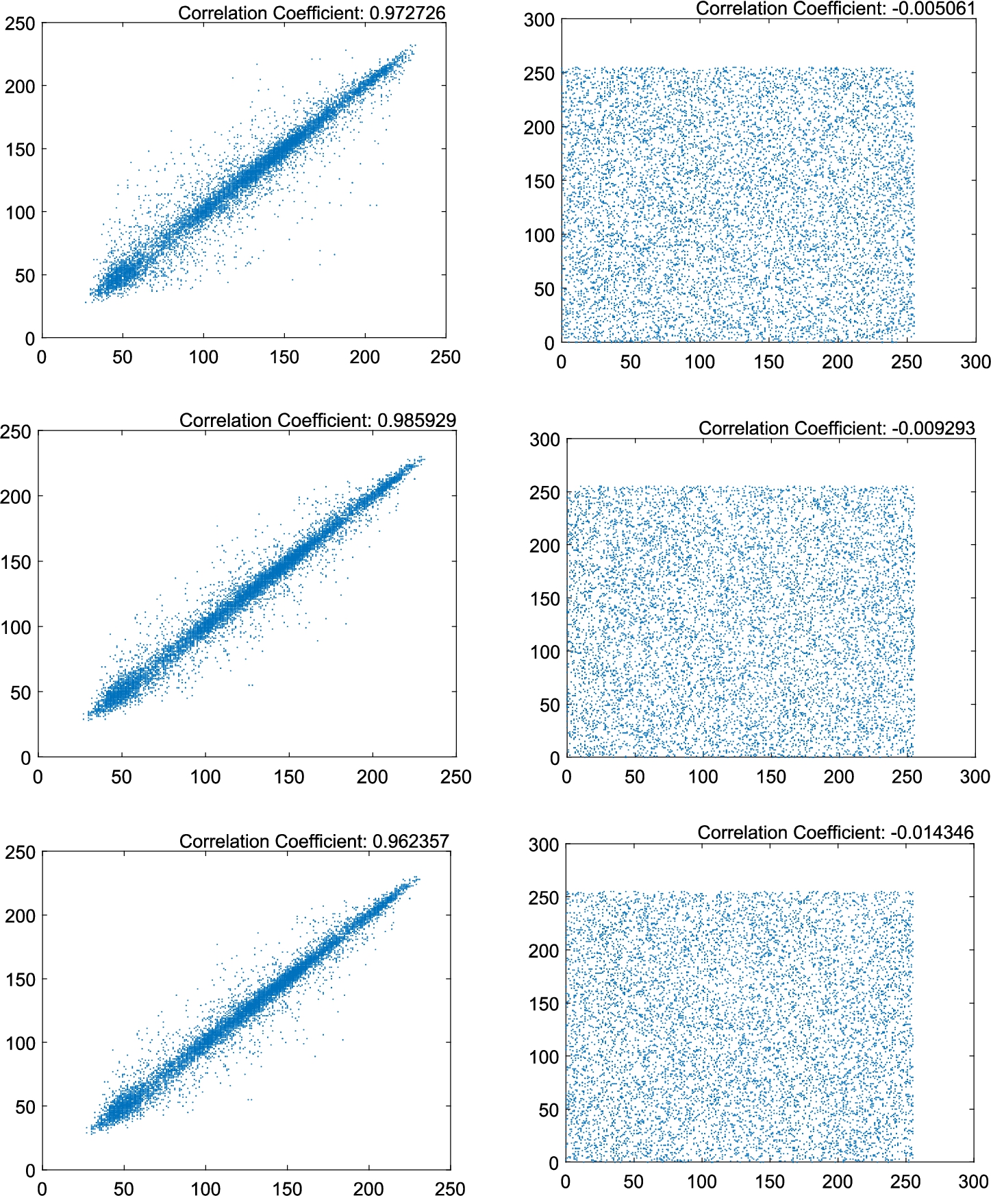
Fig. 4
Plots of $N=10000$ randomly selected adjacent pairs of pixels in the test image Lena (left), and those of a sample shadow image (right) in the horizontal, vertical and diagonal directions.
We repeat this test on 100 test images of various sizes and different structures. Each test image results in 6 shadow images. We compute the correlation coefficients between 10000 pairs of adjacent pixels in the horizontal, vertical and diagonal directions for a sample shadow image from the 6 shadow images. The obtained results are similar to those of ${H_{1}},{H_{2}},\dots ,{H_{6}}$, hence we omit them.
4.3 Entropy Analysis
Entropy (Shannon,
1951) measures the unpredictability of information content. The entropy
$H(s)$ for a source
s producing
$\ell ={2^{8}}$ distinct symbols is defined by
where
$P({s_{i}})$ is the probability of occurrence of
${s_{i}}$ in
s.
This test shows that the entropy measures
$H(s)$ for shadow images generated by the proposed scheme are close to those of truly random images i.e.
$H(s)\approx 8$. Table
3 presents the entropy measures for those images. Hence, it confirms the unpredictability of generated shadow images.
Table 3
Entropy measures for the image Lena and its six corresponding shadow images.
| Image |
Lena |
${H_{1}}$ |
${H_{2}}$ |
${H_{3}}$ |
${H_{4}}$ |
${H_{5}}$ |
${H_{6}}$ |
| $H(s)$ |
7.445507 |
7.997247 |
7.997184 |
7.997029 |
7.997582 |
7.997022 |
7.997080 |
We repeat this test on 100 test images of various sizes and different structures. Each test image results in 6 shadow images. We compute the entropy measure for a sample shadow image from the 6 shadow images. The obtained results are also close to those of truly random images, hence we omit them.
4.4 Randomness Analysis
To showcase the randomness of the shadow images generated by the proposed secret sharing scheme, we subject the six shadow images corresponding to the test image Lena to the Statistical Test Suite (STS) published by the National Institute of Standards and Technology (NIST) (Bassham
et al.,
2010). The outcome of all tests turns out to be satisfactory. Furthermore, we repeat this test on 60 shadow images each of size
$256\times 256$ obtained from running the proposed scheme on the secret image Lena for 10 different secret keys. Table
4 presents the results of each statistical test.
Table 4
Statistical Test Suite results for 60 shadow images corresponding to the test secret image Lena for ten different secret keys. The minimum pass rate for each statistical test with the exception of the random excursion (variant) test is approximately 57 for a sample size 60 sequences. The minimum pass rate for the random excursion (variant) test is approximately 29 for a sample size 32 sequences (Bassham
et al.,
2010).
| Statistical test |
P-value |
Result |
| Frequency |
0.437274 |
$60/60$ |
| Block-frequency |
0.911413 |
$59/60$ |
| Cumulative-sums (forward) |
0.772760 |
$60/60$ |
| Cumulative-sums (reverse) |
0.671779 |
$60/60$ |
| Runs |
0.014216 |
$59/60$ |
| Longest-runs |
0.568055 |
$59/60$ |
| Rank |
0.148094 |
$59/60$ |
| FFT |
0.500934 |
$60/60$ |
| Non-overlapping-templates |
0.976060 |
$60/60$ |
| Overlapping-templates |
0.407091 |
$59/60$ |
| Universal |
0.378138 |
$58/60$ |
| Approximate entropy |
0.468595 |
$60/60$ |
| Random-excursions |
0.534146 |
$32/32$ |
| Random-excursions variant |
0.350485 |
$32/32$ |
| Serial 1 |
0.437274 |
$60/60$ |
| Serial 2 |
0.949602 |
$60/60$ |
| Linear-complexity |
0.437274 |
$60/60$ |
4.5 Similarity Analysis
Similarity measures such as the Number of Pixels Change Rate (NPCR) and Unified Average Changing Intensity (UACI) (Wu
et al.,
2011) are two common measures used to study the similarity between random looking images. The NPCR and UACI are defined by
and
where
${P_{1}}$ and
${P_{2}}$ are
$M\times N$ images.
It is shown in Wu
et al. (
2011) that for gray images the ideal PSNR and UACI measures are
$99.6094\% $ and
$33.4635\% $, respectively. Furthermore, the acceptance intervals for the null hypothesis for
α-level of significance, where
$\alpha \in \{0.001,0.01,0.05\}$ are as presented in Table
5 (Wu
et al.,
2011).
Table 5
Acceptance intervals for the null hypothesis with different levels of significance (Wu
et al.,
2011).
| Parameter |
Size |
0.05-level |
0.01-level |
0.001-level |
| NPCR |
$256\times 256$ |
$[99.5693,100]$ |
$[99.5527,100]$ |
$[99.5341,100]$ |
| UACI |
$256\times 256$ |
$[33.2824,33.6447]$ |
$[33.2255,33.7016]$ |
$[33.1594,33.7677]$ |
In this test, we use the NPCR and UACI to measure the similarity between all possible pairs of shadow images corresponding to the test secret image Lena. It can be observed from the resulting measures presented in Table
6 that all measures are close to the ideal PSNR and UACI measures
$99.6094\% $ and
$33.4635\% $, respectively.
Table 6
The NPCR and UACI measures between the six shadow images corresponding to the test image Lena.
| Pair of shadow images |
NPCR |
UACI |
| $\{{H_{1}},{H_{2}}\}$ |
$99.57\% $ |
$33.53\% $ |
| $\{{H_{1}},{H_{3}}\}$ |
$99.57\% $ |
$33.46\% $ |
| $\{{H_{1}},{H_{4}}\}$ |
$99.61\% $ |
$33.52\% $ |
| $\{{H_{1}},{H_{5}}\}$ |
$99.59\% $ |
$33.37\% $ |
| $\{{H_{1}},{H_{6}}\}$ |
$99.62\% $ |
$33.48\% $ |
| $\{{H_{2}},{H_{3}}\}$ |
$99.62\% $ |
$33.58\% $ |
| $\{{H_{2}},{H_{4}}\}$ |
$99.61\% $ |
$33.42\% $ |
| $\{{H_{2}},{H_{5}}\}$ |
$99.62\% $ |
$33.53\% $ |
| $\{{H_{2}},{H_{6}}\}$ |
$99.59\% $ |
$33.54\% $ |
| $\{{H_{3}},{H_{4}}\}$ |
$99.58\% $ |
$33.55\% $ |
| $\{{H_{3}},{H_{5}}\}$ |
$99.61\% $ |
$33.47\% $ |
| $\{{H_{3}},{H_{6}}\}$ |
$99.60\% $ |
$33.60\% $ |
| $\{{H_{4}},{H_{5}}\}$ |
$99.61\% $ |
$33.64\% $ |
| $\{{H_{4}},{H_{6}}\}$ |
$99.61\% $ |
$33.49\% $ |
| $\{{H_{5}},{H_{6}}\}$ |
$99.59\% $ |
$33.47\% $ |
On the basis of the obtained measures, we conclude that the shadow images generated by the proposed scheme are random-like in comparison with one another.
4.6 Security Analysis
The security of the proposed scheme depends on keeping the secret key
${K_{0}}$ and the shadow images secure. In this proposal, the key is held at a central authority and is not shared between the participants. On the other hand, the shadow images are securely transmitted to the participant. An unauthorized person has to get hold of the secret key and at least
k shadow images to reconstruct the secret image. Now, guessing the secret key is unrealistic since it consists of six double precision floating point values in the interval
$[0,1)$ which constitute the initial states
${\mathbf{x}_{0}}$ and
${\mathbf{x}^{\prime }_{0}}$ of the cat map, and six or twelve (depending on whether the same cat matrix is used for the generation of transformation matrices and shuffling the secret image or not) positive integers for parameters of the cat matrix. Furthermore, the final stage which consists of shuffling the shares is accomplished by using the cat map with three initial states and six control parameters for each share. Moreover, Fig.
5 shows the high sensitivity of the cat map to its initial states and control parameters. This figure presents the time series plot of
${\{{x_{t}}\}_{t=0}^{100}}$ and
${\{{x^{\prime }_{i}}\}_{t=0}^{100}}$ generated by the cat map defined in Eq. (
3), where
$|{x_{0}}-{x^{\prime }_{0}}|={10^{-15}}$. It is evident from this figure that after about ten iterations the two series become far apart from each other. Nonetheless, for security issues, a chaotic map such as the cat map is usually iterated at least 200 times without considering its outputs. Likewise, guessing
k shadow images, where each shadow image consists of
$L/k$ bytes, is equivalent to guess the secret image since one has to guess
L bytes (
L is the length of the secret).
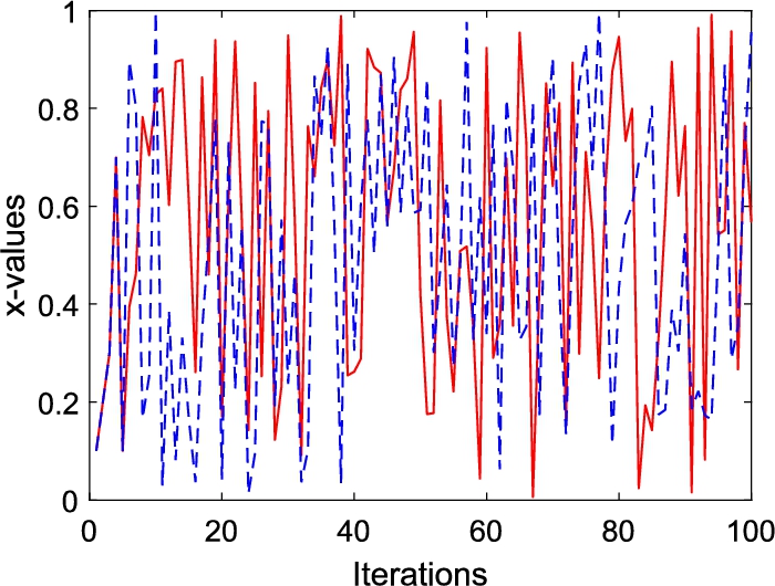
Fig. 5
Time series plot of the
x-values of the cat map defined in Eq. (
3) for two different initial states
$({x_{0}},{y_{0}},{z_{0}})$ and
$({x^{\prime }_{0}},{y_{0}},{z_{0}})$ such that
$|{x_{0}}-{x^{\prime }_{0}}|={10^{-15}}$.
In the scenario where $(k-1)$ shadow images are present, the unauthorized set of less than k participants cannot reveal any useful information about the secret image. This is due to the fact that the secret key is unknown and that one of the shadow images is missing. This can be observed from the following example. Consider a single $k\times m$ block S which can be obtained as follows: $S={(\tilde{X})^{-1}}\tilde{Y}$. Now if the $k\times k$ submatrix $\tilde{X}$ induced by the rows ${i_{1}},{i_{2}},\dots ,{i_{k}}$ of X is unknown and one of the rows of $\tilde{Y}$ is unknown, then the probability of guessing the missing elements in ${\mathbb{F}_{q}}$, where $q={2^{16}}$, correctly is about ${(1/q)^{{k^{2}}+m}}$, which renders the brute force attack infeasible for $m>100$.
4.7 Running Speed
In the proposed
$(k,n)$-threshold SIS, the generation of admissible vectors in
${\mathbb{F}_{q}^{k}}$ is image independent. Therefore, a dealer can generate the number of admissible vectors needed for the encoding of any secret image prior to the encoding process. Now, the complexity of multiplication of an
$r\times s$ matrix by an
$s\times t$ matrix is
$O(rst)$. Thus, the complexity of computing the
n shadow images is
$O(Lnk)$. Table
7 reports the running times under the aforementioned scenario for generation of shadow images for a secret image of size
${2^{s}}\times {2^{s}}$ for
$s=8,9,\dots ,13$. The reported results are obtained using MATLAB R2016a on a desktop machine with an Intel
® Core™ i7-4770 processor and 8 GB of memory, running Windows 10.
Table 7
The running times for encoding secret image of size ${2^{s}}\times {2^{s}}$ for $s=8,9,\dots ,13$ into $n=6$ shadow images using the proposed scheme with $k=4$ and $m=1024$.
| s |
8 |
9 |
10 |
11 |
12 |
13 |
| Time in seconds |
0.098432 |
0.391386 |
1.587491 |
6.390270 |
26.010420 |
106.111304 |
Furthermore, Fig.
6 shows the running times for encoding the image Lena into
n shadow images using the proposed scheme with
$k=4$ and
$m={2^{s}}$, for
$s=8,9,\dots ,15$.
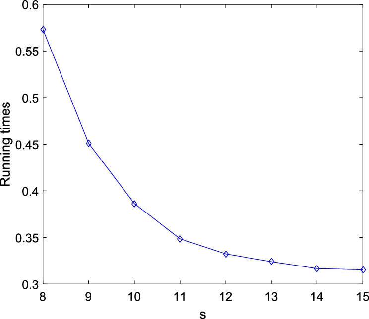
Fig. 6
The running times for generation of n shadow images (each of size $256\times 256$) by the proposed scheme where $k=4$, $n=6$ and $m={2^{s}}$.
4.8 Error-Resilient Capability
This section shows that the proposed scheme has some error-resilient capability. If some shadow images were disturbed by some noise such as salt and pepper of ratio 0.05 and 0.1, then the secret image can be reconstructed as shown in Fig.
7.
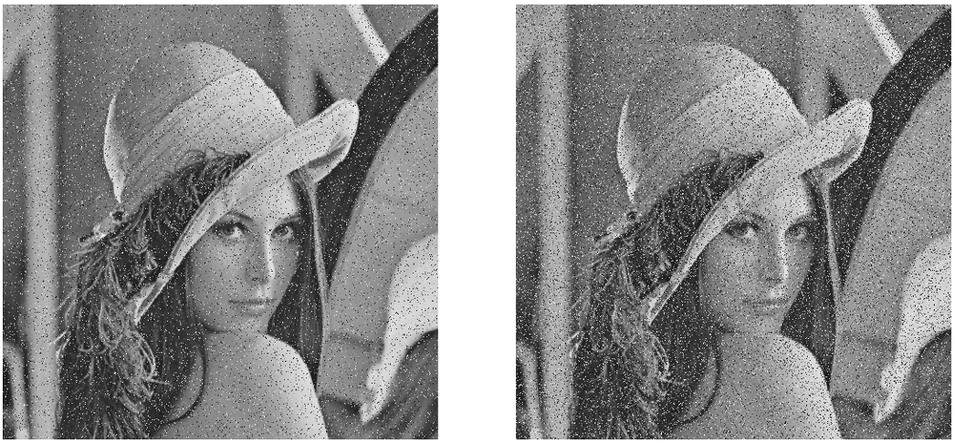
Fig. 7
The reconstructed image Lena resulting from four shadow images where one of them is subjected to salt and peppers noise with ratio: 0.05 (left) and 0.1 (right).
Furthermore, we show that if some shadow images are cropped by a certain percentage, then the secret image can still be reconstructed. Figure
8 presents a shadow image cropped by
$5\% $ and another one cropped by
$10\% $. Figure
9 (left) presents the reconstructed secret image Lena resulting from four shadow images where one of them is cropped by
$5\% $, whereas Fig.
9 (right) presents the reconstructed secret image Lena resulting from four shadow images where one of them is cropped by
$10\% $. Thus, it is evident that the proposed scheme is resistant to the cropping attack.
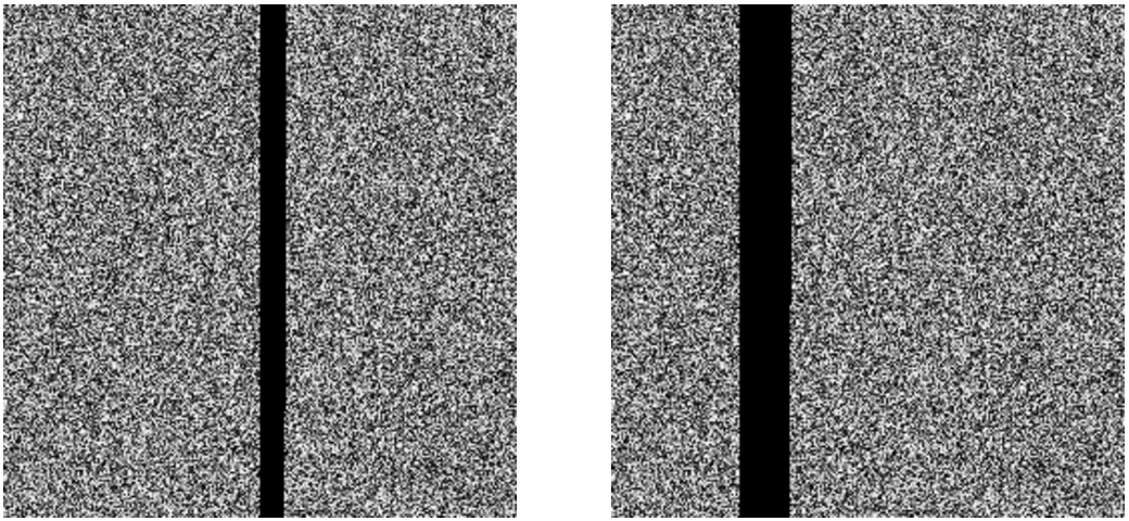
Fig. 8
A shadow image cropped by $5\% $ (left) and another one cropped by $10\% $ (right).
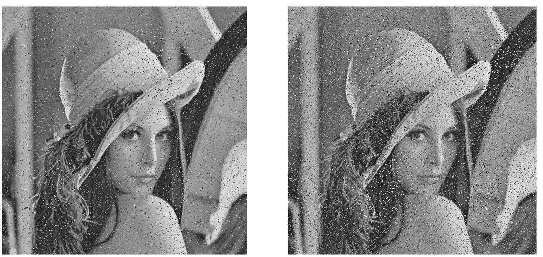
Fig. 9
The reconstructed image Lena resulting by the proposed scheme from four shadow images where one shadow image is subjected to cropping by $5\% $ (left) and $10\% $ (right).
5 Comparison with Existing Work
In this section we compare the performance of the proposed approach, referred to by Pr-SIS, with few existing
$(k,n)$-SIS schemes: TL (Thien and Lin,
2002), Wu (
2013), KG (Kanso and Ghebleh,
2017), KE (Kabirirad and Eslami,
2018) and GK (Ghebleh and Kanso,
2018). All comparisons are performed with
$(k,n)=(2,4)$ with the secret image Pirate of size
$512\times 512$ presented in Fig.
10. The sizes of the generated shadows images are presented in Table
8.
In Table
9, we present the correlation coefficients between
$N=10000$ pairs of randomly selected adjacent pixels in the horizontal, vertical and diagonal directions of sample shadow images generated by TL (Thien and Lin,
2002), Wu (Wu,
2013), KG (Kanso and Ghebleh,
2017), KE (Kabirirad and Eslami,
2018), GK (Ghebleh and Kanso,
2018) and Pr-SIS. It is evident from this table that all schemes generate shadow images almost free of any correlation between adjacent pixels.
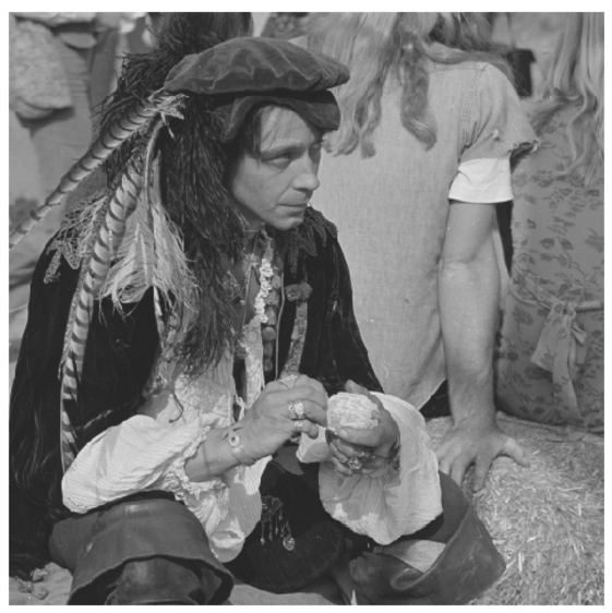
Fig. 10
The test image Pirate of size $512\times 512$.
Table 8
The size of shadow images generated by the scheme under comparison.
| Scheme |
Size of shadow image |
Lossy |
| TL (Thien and Lin, 2002) |
$L/k$ |
Yes |
| Wu (Wu, 2013) |
$L/k$ |
Yes |
| KG (Kanso and Ghebleh, 2017) |
$L/k$ |
Yes |
| KE (Kabirirad and Eslami, 2018) |
L |
No |
| GK (Ghebleh and Kanso, 2018) |
$L/(k-1)$ |
Yes |
| Pr-SIS |
$L/k$ |
No |
Table 9
Correlation coefficients of pairs of adjacent pixels in sample shadow images generated by (i) TL, (ii) Wu, (iii) KG, (iv) GK and (v) Pr-SIS.
| Scheme |
Horizontal |
Vertical |
Diagonal |
| TL (Thien and Lin, 2002) |
0.001429 |
−0.002693 |
−0.012811 |
| Wu (Wu, 2013) |
0.015723 |
−0.008210 |
0.006800 |
| KG (Kanso and Ghebleh, 2017) |
−0.004502 |
−0.007861 |
−0.008209 |
| KE (Kabirirad and Eslami, 2018) |
−0.085000 |
0.050000 |
−0.189000 |
| GK (Ghebleh and Kanso, 2018) |
−0.004358 |
−0.007642 |
−0.007148 |
| Pr-SIS |
−0.003981 |
−0.008036 |
0.009603 |
Table
10 presents the entropy measures of sample shadow images of the schemes under comparison.
Table 10
The entropy measures of sample shadow images generated by the scheme under comparison.
| Scheme |
$H(s)$ |
| TL (Thien and Lin, 2002) |
7.901762 |
| Wu (Wu, 2013) |
7.943923 |
| KG (Kanso and Ghebleh, 2017) |
7.908187 |
| KE (Kabirirad and Eslami, 2018) |
7.999300 |
| GK (Ghebleh and Kanso, 2018) |
7.999249 |
| Pr-SIS |
7.998559 |
Table
11 presents the mean absolute difference of the secret image Pirate and the reconstructed image by the schemes under comparison. This table also presents the Peak Signal to Noise Ratio (PSNR) and The Structural Similarity (SSIM) measures between the secret image and the reconstructed one (Wang
et al.,
2004).
Table 11
The number of errors in the reconstructed image, the mean absolute difference between the two images as well as their PSNR and SSIM measures.
| Scheme |
Number of modified pixels |
Number of modified LSB |
Mean absolute difference |
PSNR |
SSIM |
| TL (Thien and Lin, 2002) |
39360 |
79205 |
0.735153 |
42.528821 |
0.999906 |
| Wu (Wu, 2013) |
113 |
218 |
0.006897 |
57.703019 |
0.999948 |
| KG (Kanso and Ghebleh, 2017) |
38350 |
38350 |
0.1462946 |
56.478549 |
0.999996 |
| KE (Kabirirad and Eslami, 2018) |
0 |
0 |
0 |
∞ |
1.000000 |
| GK (Ghebleh and Kanso, 2018) |
2729 |
2729 |
0.010410 |
67.956168 |
0.999996 |
| Pr-SIS |
0 |
0 |
0 |
∞ |
1.000000 |
On the basis of the above results it is evident that the proposed scheme is competitive with existing schemes. Many existing secret image sharing schemes use arithmetics in the finite files
${\mathbb{F}_{q}}$ where
q is a suitable prime. This yields in the need for truncation of values and, in turn, in all these schemes being lossy, and hence incapable of applications where the secret is sensitive. The proposed scheme, on the other hand, is defined on the field
${\mathbb{F}_{q}}$ where
q is a power of 2. This choice is more suitable for handling binary data since with a proper choice of
q one can avoid truncations of values. As shown in Table
8, among the schemes in comparison, only KE is lossless, but it is at a clear disadvantage to the proposed scheme Pr-SIS since each shadow image produced by KE has the same size as the original secret image.
6 Concluding Remarks
In this research, we propose a lossless linear algebraic $(k,n)$-SIS which associates a vector ${\mathbf{v}_{i}}$ to the ith participant in the vector space ${\mathbb{F}_{q}^{k}}$, where q is a power of 2. Admissibility conditions are imposed on the vectors ${\mathbf{v}_{i}}$ to satisfy the threshold property of secret sharing. The scheme is shown to possess a number of characteristics such as robustness against standard statistical attacks, high level of security including sensitivity to its secret key, resilience to errors in shadow images, and reduction in the size of shadow images with respect to the size of the secret image. Another feature of the scheme is being lossless, which enables applications to digital media other than raw images. For example, the proposed scheme can be used for sharing textual data, JPEG images, video, etc.
The proposed scheme is very fast provided the admissibility of the transformation matrix is verified beforehand. This step is independent of the secret image and does not present any security risks to the process of secret image sharing. On the other hand, checking admissibility is costly in general and could be considered as a disadvantage of the proposed scheme if it is not performed independently of the secret sharing itself. Processing time and shadow image size can be further reduced if the proposed scheme is used in conjunction with image compression algorithms such as those based on vector quantization.

