Informatica logo


Login Register

  1. Home
  2. Issues
  3. Volume 30, Issue 3 (2019)
  4. Fuzzifier Selection in Fuzzy C-Means fro ...

Informatica

Information Submit your article For Referees Help ATTENTION!
  • Article info
  • Full article
  • Related articles
  • Cited by
  • More
    Article info Full article Related articles Cited by

Fuzzifier Selection in Fuzzy C-Means from Cluster Size Distribution Perspective
Volume 30, Issue 3 (2019), pp. 613–628
Kaile Zhou   Shanlin Yang  

Authors

 
Placeholder
https://doi.org/10.15388/Informatica.2019.221
Pub. online: 1 January 2019      Type: Research Article      Open accessOpen Access

Received
1 August 2018
Accepted
1 March 2019
Published
1 January 2019

Abstract

Fuzzy c-means (FCM) is a well-known and widely applied fuzzy clustering method. Although there have been considerable studies which focused on the selection of better fuzzifier values in FCM, there is still not one widely accepted criterion. Also, in practical applications, the distributions of many data sets are not uniform. Hence, it is necessary to understand the impact of cluster size distribution on the selection of fuzzifier value. In this paper, the coefficient of variation (CV) is used to measure the variation of cluster sizes in a data set, and the difference of coefficient of variation (DCV) is the change of variation in cluster sizes after FCM clustering. Then, considering that the fuzzifier value with which FCM clustering produces minor change in cluster variation is better, a criterion for fuzzifier selection in FCM is presented from cluster size distribution perspective, followed by a fuzzifier selection algorithm called CSD-m (cluster size distribution for fuzzifier selection) algorithm. Also, we developed an indicator called Influence Coefficient of Fuzzifier ($\mathit{ICF}$) to measure the influence of fuzzifier values on FCM clustering results. Finally, experimental results on 8 synthetic data sets and 4 real-world data sets illustrate the effectiveness of the proposed criterion and CSD-m algorithm. The results also demonstrate that the widely used fuzzifier value $m=2$ is not optimal for many data sets with large variation in cluster sizes. Based on the relationship between ${\mathit{CV}_{0}}$ and $\mathit{ICF}$, we further found that there is a linear correlation between the extent of fuzzifier value influence and the original cluster size distributions.

1 Introduction

Clustering (Jain, 2010; Hartigan, 1975; Khemchandani and Pal, 2019) is an unsupervised learning process to partition a given data set into clusters based on similarity/dissimilarity functions, such that the data objects partitioned in the same cluster are as similar as possible, while those in different clusters are dissimilar at the same time. Currently, there have been various clustering methods that were proposed and applied in many areas (Olde Keizer et al., 2016; Benati et al., 2017; Truong et al., 2017; Pham et al., 2018; Motlagh et al., 2019; Borg and Boldt, 2016; Mokhtari and Salmasnia, 2015).
For crisp clustering method, like k-means (MacQueen, 1967; Mehdizadeh et al., 2017) or hierarchical clustering method (Johnson, 1967), each data object can only be partitioned into one cluster. While fuzzy c-means (FCM) (Bezdek et al., 1984; Zhao et al., 2013) introduced the concept of membership degree so that each object can belong to two or more clusters with a certain membership degree value. FCM is the extension of hard k-means clustering, and the rich information conveyed by the membership degree and fuzzifier in FCM further expanded its application areas. FCM algorithm was first proposed by Dunn and generalized by Bezdek (Dunn, 1973; Bezdek, 1981), and it has become a popular and widely used fuzzy clustering method in pattern recognition (Ahmed et al., 2002; Dembélé and Kastner, 2003; Park, 2009; Hou et al., 2007).
However, the fuzzifier, also known as the weighting exponent or fuzziness parameter in FCM, is an important parameter in FCM which can significantly influence the performance of FCM clustering (Pal and Bezdek, 1995). There have been considerable research efforts that focused on the selection of fuzzifier, and many suggestions have been proposed (Cannon et al., 1986; Hall et al., 1992; Shen et al., 2001; Ozkan and Turksen, 2004, 2007; Wu, 2012). However, there is still not one generally accepted criterion and few theoretical guides for the selection of fuzzifier in FCM (Fadili et al., 2001). In many cases, users subjectively select the value of fuzzifier while using FCM clustering.
In addition, the distributions of many data sets are not uniform in practical applications (Wu et al., 2012). It has been demonstrated that clustering performance is always affected by data distributions (Xiong et al., 2009; Wu et al., 2009c). In our previous work (Zhou and Yang, 2016), we have also found that FCM has the uniform effect similar to k-means clustering. The clustering results of FCM can be significantly influenced by the cluster size distributions. Therefore, to improve the performance of FCM for data sets with different cluster size distributions, it is important to select the appropriate value of fuzzifier. In this study, a new fuzzifier selection criterion and a corresponding algorithm called CSD-m algorithm are proposed from the perspective of cluster size distribution. The cluster size distribution mainly refers to the variation of cluster sizes. First, we use the coefficient of variance (CV) to measure the variation of data in cluster sizes. Then, the values of DCV, which indicate the change of variation in cluster sizes after FCM clustering, are calculated iteratively with different fuzzifier values within an initial search interval. Finally, according to the minimum absolute value of DCV, the optimal value of fuzzifier is determined. Our experiments on both synthetic data sets and real-world data sets illustrate the effectiveness of the proposed criterion and CSD-m algorithm. The experimental results also reveal that the widely used fuzzifier value $m=2$ is not optimal for many data sets, especially for data sets with large variation in cluster sizes.
The fuzzifier, denoted as m in FCM, is an important parameter which can significantly influence the performance of FCM clustering. Currently, there have been considerable studies on fuzzifier selection. Bezdek proposed a range interval of fuzzifier, $1.1\leqslant m\leqslant 5$, based on experience (Bezdek, 1981). Pal and Bezdek presented a heuristic criteria for the selection of optimal fuzzifier value, and the interval they suggested was $[1.5,2.5]$ (Pal and Bezdek, 1995). They also pointed out that the median, namely $m=2$, can be selected when there is no other specific constraints. Some studies (Cannon et al., 1986; Hall et al., 1992; Shen et al., 2001) presented the similar suggestion as the work of Pal and Bezdek (1995). In addition, Bezdek studied the physical interpretation of FCM when $m=2$ and pointed out that $m=2$ was the best selection (Bezdek, 1976). The study of Bezdek et al. further demonstrated that the value of m should be greater than $n/(n-2)$, where n is the total number of sample objects (Bezdek et al., 1987). Based on their work of word recognition, Chan and Cheung suggested that the value range of m should be $[1.25,1.75]$ (Chan and Cheung, 1992). However, Choe and Jordan pointed out that the performance of FCM is not sensitive to the value of m based on the fuzzy decision theory (Choe and Jordan, 1992). Ozkan and Turksen presented an entropy assessment for m considering the uncertainty contained (Ozkan and Turksen, 2004). To obtain the uncertainty generated by m in FCM, Ozkan and Turksen also identified the upper and lower values of m as 1.4 and 2.6, respectively, (Ozkan and Turksen, 2007). Wu proposed a new guideline for the selection of m based on a robust analysis of FCM, and suggested implementing FCM with $m\in [1.5,4]$ (Wu, 2012).
In summary, there is still not one widely accepted criterion and little theoretical support for the selection of fuzzifier in FCM (Pal and Bezdek, 1995; Yu et al., 2004). In most practical applications, the value of fuzzifier is always subjectively selected by users, and $m=2$ is the most common selection (Pal and Bezdek, 1995; Cannon et al., 1986; Hall et al., 1992; Shen et al., 2001). Indeed, this selection may not be always the optimal, and inappropriate selection of fuzzifier value can significantly affect the clustering results of FCM. Additionally, few of the above researches have focused on the cluster size distribution while studying the related issue of fuzzifier selection. The characteristics of cluster size distribution may have an impact on the performance of FCM clustering. Fuzzifier is a key parameter that influences the clustering results of FCM. Furthermore, in some studies, only the range intervals of empirical reference values were presented without specific criterion and method for the selection of optimal fuzzifer value in practical applications. Therefore, the motivation of this study is to explore the influence and measure the influence extent of fuzzifier value on FCM clustering results, and further investigate the fuzzifier selection from a cluster size distribution perspective. The main contributions of this study are as follows. First, the mechanism that fuzzifier influences the FCM clustering result is revealed. Second, we point out that the widely used fuzzifier value $m=2$ is not optimal for many data sets with large variation in cluster sizes. Third, a criterion and a CSD-m algorithm for fuzzifier selection in FCM is presented from cluster size distribution perspective.
We note that, for a given data set, “data distribution” typically means many aspects of the characteristics, such as the shapes, densities and dimensions. While the focus of this study is the cluster size distributions of data sets. So we use cluster size distribution to represent the variation in cluster sizes of a data set.
The remainder of this paper is organized as follows. The FCM clustering algorithm is briefly reviewed in Section 2. In Section 3, we propose the fuzzifier selection criterion from cluster size distribution perspective and the corresponding algorithm called CSD-m algorithm. Experimental results and discussion are presented in Section 4. Finally, conclusions are made in Section 5.

2 FCM Clustering

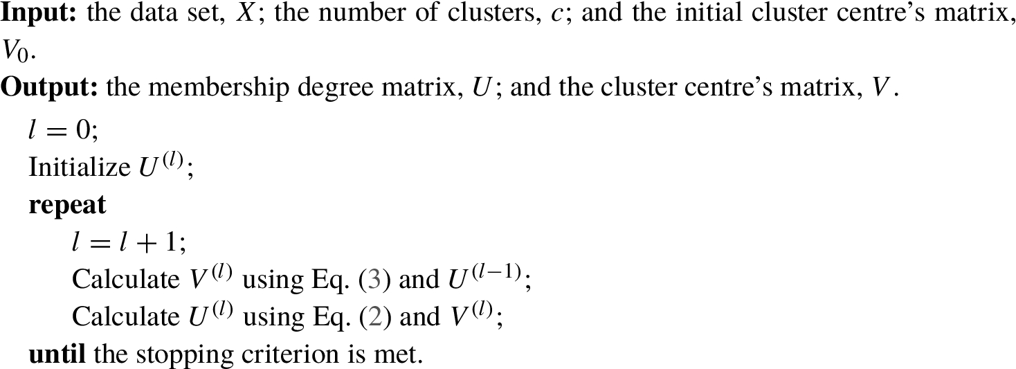
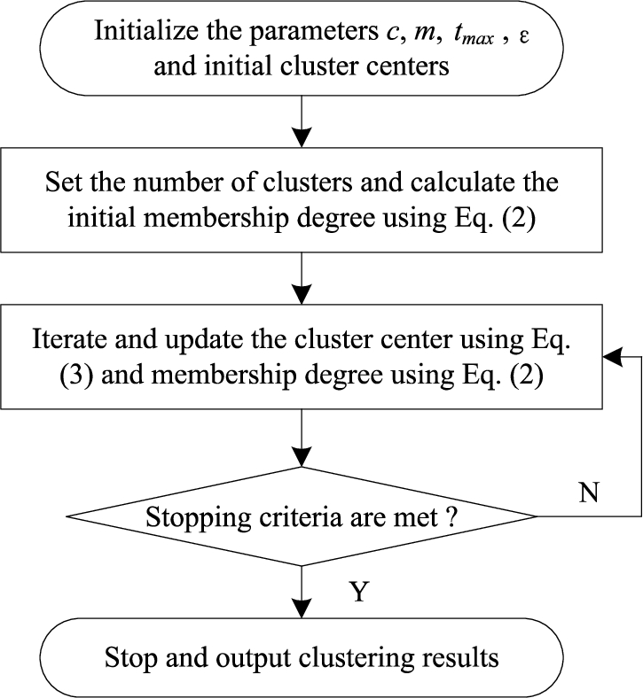
FCM algorithm (Bezdek et al., 1984; Bezdek, 1981) starts with determining the number of clusters followed by guessing the initial cluster centres. Then every sample point is assigned a membership degree for each cluster. Each cluster centre’s point and corresponding membership degrees are updated iteratively by minimizing the objective functions until the stopping criteria are met. The stopping criteria mainly include the iterations t reach the maximum number ${t_{\max }}$, or the difference of the cluster centres between two consecutive iterations is within a small enough threshold ε, i.e. $\| {v_{i,t}}-{v_{i,t-1}}\| \leqslant \varepsilon $. The objective function of FCM algorithm is defined as:
(1)
\[ {J_{m}}(U,V)={\sum \limits_{i=1}^{c}}{\sum \limits_{j=1}^{n}}{\mu _{ij}^{m}}{d_{ij}^{2}},\]
where U is the membership degree matrix. V represents the cluster centre’s matrix. n is the total number of data objects in the data set. c is the number of clusters. m is the fuzzifier. ${\mu _{ij}}$ is the membership degree of the jth data object ${x_{j}}$ to the ith cluster ${C_{i}}$. ${v_{i}}$ is the cluster centre of ${C_{i}}$. ${d_{ij}^{2}}$ is the squared Euclidean distance between ${x_{j}}$ and the cluster centre ${v_{i}}$, and ${d_{ij}^{2}}=\| {x_{j}}-{v_{i}}{\| ^{2}}$.
In the iterative procedure, membership degree ${\mu _{ij}}$ and the cluster centres ${v_{i}}$ are updated by:
(2)
\[\begin{aligned}{}& {\mu _{ij}}=\frac{1}{{\textstyle\textstyle\sum _{k=1}^{c}}{(\frac{{d_{ij}}}{{d_{kj}}})^{\frac{2}{m-1}}}},\end{aligned}\]
(3)
\[\begin{aligned}{}& {v_{i}}=\frac{{\textstyle\textstyle\sum _{j=1}^{n}}{\mu _{ij}^{m}}{x_{j}}}{{\textstyle\textstyle\sum _{j=1}^{n}}{\mu _{ij}^{m}}},\end{aligned}\]
where ${\mu _{ij}}$ satisfies
(4)
\[\begin{aligned}{}& {\mu _{ij}}\in [0,1],\end{aligned}\]
(5)
\[\begin{aligned}{}& {\sum \limits_{i=1}^{c}}{\mu _{ij}}=1,\hspace{1em}\forall j=1,\dots ,n,\end{aligned}\]
(6)
\[\begin{aligned}{}& 0<{\sum \limits_{j=1}^{n}}{\mu _{ij}}<n,\hspace{1em}\forall i=1,\cdots \hspace{0.1667em},c.\end{aligned}\]
The meanings of the symbols in Eq. (2) to Eq. (6) are the same as those in Eq. (1).
The basic FCM algorithm is briefly reviewed as Algorithm 1.
info1224_g001.jpg
Algorithm 1
Fuzzy c-means (FCM)
The flowchart of FCM algorithm can be shown in Fig. 1.
info1224_g002.jpg
Fig. 1
Flow chart of FCM clustering.

3 Fuzzifier Selection Method from Cluster Size Distribution Perspective

3.1 Measure of Cluster Size Distribution

The coefficient of variance ($\mathit{CV}$) (Papoulis, 1990) in statistics can be used as a measure for the variation in cluster sizes of a data set (Xiong et al., 2009; Wu et al., 2009c).
Definition 1 (Coefficient of Variance, $\mathit{CV}$).
$\mathit{CV}$ is the ratio of the standard deviation to the mean of cluster sizes, which is calculated as follows:
(7)
\[\begin{aligned}{}& \bar{n}=\frac{1}{c}{\sum \limits_{i=1}^{c}}{n_{i}},\end{aligned}\]
(8)
\[\begin{aligned}{}& \sigma =\sqrt{\frac{{\textstyle\textstyle\sum _{i=1}^{c}}{({n_{i}}-\bar{n})^{2}}}{c-1}},\end{aligned}\]
(9)
\[\begin{aligned}{}& \mathit{CV}=\frac{\sigma }{\bar{n}},\end{aligned}\]
where c is the number of clusters, ${n_{i}}$ is the number of objects in cluster ${C_{i}}$, $\bar{n}$ is the average size of all the clusters, and σ is the standard deviation of the cluster size distribution.
$\mathit{CV}$ can be used to measure the distribution of cluster sizes since it is the ratio of the standard deviation and the average value of cluster sizes. $\mathit{CV}$ is a dimensionless measure, which makes it more effective in measuring cluster size distributions. Generally, the larger the $\mathit{CV}$ value is, the greater the variability is in the data.
Definition 2 (DCV).
${\mathit{CV}_{0}}$ is the $\mathit{CV}$ value of the original “true” clusters, and ${\mathit{CV}_{1}}$ is the CV value of the clustering result partitioned by FCM. DCV is defined as the change of variation in cluster sizes after FCM clustering (Zhou and Yang, 2016; Wu et al., 2009a, 2009b).
(10)
\[ \mathit{DCV}={\mathit{CV}_{0}}-{\mathit{CV}_{1}}.\]
From the perspective of cluster size distribution, a clustering partition which results in minor change of variation in cluster sizes (i.e. a smaller absolute value of $\mathit{DCV}$) refers to a steady state of clustering result. Based on this, we propose a criterion for fuzzifier selection in FCM from cluster size distribution perspective.
Criterion 1 (Fuzzifier selection criterion from cluster size distribution perspective).
In a certain range of fuzzifier values, the fuzzifier value with which the FCM clustering can result in the minimum absolute value of DCV is the optimal selection.
We note that DCV is more of an indication of reaching steady state of the clustering process, and it does not necessarily indicate a better partition result. However, in FCM clustering with different fuzzifier values, for a specific data set, the distribution changes are mainly reflected in the cluster sizes. Therefore, to a certain extent, we can say that criterion 1 is valid.

3.2 CSD-m Algorithm for Fuzzifer Selection

Based on the fuzzifier selection criterion from cluster size distribution perspective, we propose a fuzzifier selection algorithm considering the change of variation in cluster sizes. The algorithm is called cluster size distribution based fuzzifier m selection algorithm (CSD-m algorithm), as described in Algorithm 2.
info1224_g003.jpg
Algorithm 2
CSD-m algorithm
The flow chart of the proposed CSD-m algorithm is shown in Fig. 2.
info1224_g004.jpg
Fig. 2
Flow chart of the CSD-m algorithm.
The DCV measure for the change of variation in cluster sizes after FCM clustering and the search process of fuzzifier values in a range interval are added to the traditional FCM algorithm to form the CSD-m algorithm. Apart from the number of clusters and the initial cluster centres, the search interval of fuzzifier values is also needed as the input of CSD-m algorithm. This interval can be determined according to the existing suggestions, as discussed in Section 2. The key steps of CSD-m algorithm are the calculation of CV values partitioned by FCM clustering with different fuzzifier values, and the comparison of absolute DCV values. Through the iterations, the optimal value of fuzzifier is obtained when $|DCV|$ reaches its minimum.

4 Experimental Study

4.1 Experimental Setup

In the experiments, 8 synthetic data sets and 4 real-world data sets are used to demonstrate the effectiveness of our proposed fuzzifier selection criterion and the CSD-m algorithm. The experimental tool is Matalb R2012b. Based on the existing research on fuzzifier selection, the search range of fuzzifier is set to $[1.2,3.0]$. Taking into account the efficiency of the CSD-m algorithm, we set $\Delta m=0.2$. The maximum number of iterations and the termination threshold of FCM are the default values, namely, 100 and 1e−5, respectively. Also, due to the randomness of initial cluster centres in FCM, we run the algorithm ten times with each m value for each data set, and the average values are obtained as the final results.
The synthetic data sets are named SDXYYYY, in which “SD” refers to synthetic data set, “X” refers to the dimension of the data set, and “YYYY” indicates the number of data objects in the data set. The synthetic data sets are randomly generated by using the $\mathit{nngenc}$ function in Matlab R2012b with different bounds and standard deviation parameters. We control the parameters of $\mathit{nngenc}$ function, such that all of these synthetic data sets have great variation in cluster sizes. The generation parameters of the 8 synthetic data sets are shown in Table 1.
Table 1
Generation parameters of the synthetic datasets.
Dataset No. of clusters No. of dimensions Cluster centre bounds Std. of each cluster
SD21000 2 2 (2, 4); (4, 4) 0.4; 0.3
SD20550 3 2 (1, 1); (2, 3); (4, 2) 0.4; 0.4; 0.4
SD21800 4 2 (2, 2); (2, 7); (5, 2); (6, 7) 0.7; 0.8; 0.4; 0.5
SD21950 5 2 (2, 2); (2, 6); (6, 2); (6, 6); (4, 4) 0.5; 0.4; 0.4; 0.4; 0.6
SD31500 2 3 (2, 2, 2); (4, 4, 3) 0.5; 0.5
SD32050 3 3 (2, 2, 2); (4, 4, 3); (5, 3, 2) 0.6; 0.4; 0.4
SD32800 4 3 (2, 2, 2); (4, 4, 3); (5, 3, 2); (6, 6, 4) 0.7; 0.4; 0.4; 0.7
SD34000 5 3 (2, 2, 2); (4, 4, 3); (5, 3, 2); (6, 6, 4); (6, 7, 2) 0.7; 0.4; 0.5; 0.6; 0.5
The distributions of the 8 synthetic data sets are shown in Fig. 3.
info1224_g005.jpg
Fig. 3
Distributions of the synthetic data sets.
The four real-world data sets are from different areas in the UCI Machine Learning Repository (Bache and Lichman, 2013). The abalone data set is a real-world data set to predict the age of abalone from physical measurements. The balance-scale data set contains information about balance scale weight and distance. The breast-cancer data set includes the original Wisconsin breast cancer related information of 699 instances. The page-blocks data set measures the blocks of the page layout of a document that has been detected by a segmentation process.
Some key characteristics of the experimental data sets are summarized in Table 2.
Table 2
Some characteristics of experimental data sets.
Data sets # Objects # Features # classes MinSize MaxSize AvgSize ${\mathit{CV}_{0}}$
Synthetic data sets SD21000 1000 2 2 100 900 500 1.131
SD20550 550 2 3 50 350 183 0.833
SD21800 1800 2 4 200 950 450 0.754
SD21950 1950 2 5 100 1200 390 1.176
SD31500 1500 3 2 200 1300 750 1.037
SD32050 2050 3 3 200 1500 683 1.041
SD32800 2800 3 4 200 1500 700 0.849
SD34000 4000 3 5 200 2000 800 0.923
Real-world data sets abalone 4177 8 29 1 689 144 1.414
balance-scale 625 4 3 49 288 208 0.662
breast-cancer 699 10 8 17 367 87 1.320
pageblocks 5473 10 5 28 4913 1095 1.953
In Table 1, “# objects” represents the total number of data objects in the data set. “# features” is the number of attributes of the data. “# classes” refers to the number of clusters in the data.

4.2 Results and Discussion

The clustering results of both the 2-D and 3-D synthetic data sets can be visualized so that we can directly understand the effect of different fuzzifier values on the clustering results. For simplicity, we only present the FCM clustering results with the popular fuzzifier values of $m=2.0$ on the 8 synthetic data sets, as shown in Fig. 4.
info1224_g006.jpg
Fig. 4
Clustering partitions of FCM with fuzzifier value $m=2.0$.
The clustering results on four synthetic data sets show that the smaller the fuzzifier value is, the better the clustering result is. With the increase of fuzzifier value, the small clusters in the data sets tend to merge with part of the larger clusters.
The clustering results of all the experimental data sets with different fuzzifier values are presented in Table 3.
Then, based on the ${\mathit{CV}_{1}}$ values in Table 3, we calculate the DCV values with different fuzzifier values on all of the 12 experimental data sets. The changes of DCV values on all the experimental data sets with different fuzzifier values are shown in Fig. 5.
Table 3
Clustering results of all the experimental data sets with different fuzzifier values.
Data sets ${\mathit{CV}_{0}}$ ${\mathit{CV}_{1}}$
$m=1.2$ $m=1.4$ $m=1.6$ $m=1.8$ $m=2.0$ $m=2.2$ $m=2.4$ $m=2.6$ $m=2.8$ $m=3.0$
Synthetic data sets SD21000 1.131 1.095 1.081 1.064 1.027 1.001 0.950 0.857 0.713 0.619 0.580
SD20550 0.833 0.824 0.824 0.824 0.819 0.819 0.819 0.819 0.814 0.814 0.814
SD21800 0.754 0.738 0.736 0.736 0.735 0.732 0.732 0.732 0.732 0.730 0.728
SD21950 1.176 1.075 1.072 1.069 1.063 0.640 0.623 0.610 0.600 0.593 0.589
SD31500 1.037 1.033 1.033 1.033 1.031 1.030 1.030 1.030 1.020 1.015 1.005
SD32050 1.041 0.162 0.162 0.162 0.163 0.168 0.180 0.187 0.188 0.187 0.194
SD32800 0.849 0.739 0.790 0.725 0.716 0.704 0.170 0.171 0.174 0.179 0.180
SD34000 0.923 0.489 0.308 0.307 0.306 0.306 0.305 0.303 0.301 0.299 0.299
Real-world data sets abalone 1.414 0.661 0.564 0.558 0.509 0.511 0.453 0.406 0.355 0.378 0.354
balance-scale 0.662 0.183 0.083 0.030 0.023 0.145 0.316 0.211 0.294 0.227 0.287
breast-cancer 1.320 0.929 0.966 0.978 0.802 0.747 0.858 0.901 0.850 0.831 0.879
pageblocks 1.953 1.547 1.547 1.564 1.518 1.485 1.562 1.474 1.277 1.233 1.276
info1224_g007.jpg
Fig. 5
The m–$\mathit{DCV}$ relationship on all the experimental data sets.
According to the criterion of fuzzifier selection, we can see from Fig. 5 that the optimal values of fuzzifier determined by the CSD-m algorithm on different data sets are not the same. Furthermore, the relationships between m and DCV values are not the simple linear relationship. Nevertheless, for most data sets which have large variation in clusters sizes, smaller fuzzifier values tend to produce better clustering results. Generally, small clusters tend to merge with parts of the large clusters with the increase of fuzzifier values, as illustrated in Fig. 2.
From the obtained DCV values, the optimal fuzzifier values of the 12 data sets are shown in Fig. 6.
info1224_g008.jpg
Fig. 6
Optimal fuzzifier values obtained for the experimental data sets.
As we can see from Fig. 6, the widely accepted and applied fuzzifier value in FCM, namely $m=2$, is not an optimal value for most of the data sets. Interestingly, we find that for most of the data sets, the smaller fuzzifier, $m=1.2$, is an optimal value.
As we know, the inappropriate selection of fuzzifier value can significantly influence the clustering results of FCM. From Fig. 3, we can also see that the extents to which the clustering partitions are influenced by the fuzzifier values are different. Therefore, we define an indicator called Influence Coefficient of Fuzzifier ($\mathit{ICF}$) based on the change of ${\mathit{CV}_{1}}$ values and the threshold of fuzzifier parameter m, to measure the influence of fuzzifier parameter m on FCM clustering results. The ICF indicator is defined as
(11)
\[ \mathit{ICF}=\frac{|\Delta {\mathit{CV}_{1}}|}{\Delta m}.\]
With the change of m, if the change of ${\mathit{CV}_{1}}$ is large, then the value of $\mathit{ICF}$ indicator is large. It demonstrates that the influence of m on FCM clustering is large. In contrast, within the similar threshold of m, a smaller $\Delta {\mathit{CV}_{1}}$ value indicates the influence of m on FCM clustering is relatively small.
We choose the range of m values from 1.2 to 3.0, and then the $\mathit{ICF}$ values on the 12 experimental data sets can be obtained. To discover the different influences of fuzzifier value on different data sets, the relationship between $\mathit{ICF}$ values and ${\mathit{CV}_{0}}$ values are fitted as shown in Fig. 7.
info1224_g009.jpg
Fig. 7
Relationship between $\mathit{ICF}$ and ${\mathit{CV}_{0}}$.
From Fig. 7, we can see that there exists a linear relationship between ${\mathit{CV}_{0}}$ and $\mathit{ICF}$. The linear regression equation, $y=0.64x-0.47$, reveals an interesting relationship between the influence extent of fuzzifier value and the original cluster size distributions. It demonstrates that the influences of fuzzifier value on FCM clustering results are relatively small on data sets with small variation in sizes. However, for data sets with large variation in cluster sizes, it is of particular importance to pay attention to the great influence of fuzzifier value on FCM clustering.
We also note that to a certain extent, the very small clusters in a data set can be regarded as noises and outliers. It has been recognized that the outliers can affect the performance of FCM. To address this problem, some existing studies have suggested to modify the Euclidean distance of FCM (Hathaway et al., 2000; Kersten, 1999). However, the focus of this study is the influence of fuzzifer values in FCM. Without modifying the FCM algorithm itself, the small clusters can be effectively identified with an appropriate fuzzifier value using our proposed CSD-m algorithm. Therefore, our method also contributes to the identification of noises and outliers when using traditional FCM clustering.

5 Conclusion

The fuzzifier in FCM is an important parameter which can significantly influence the clustering results of FCM. Considering that the distribution of many data sets are not uniform in practical applications, we propose a new criterion and the corresponding algorithm called CSD-m algorithm for the selection of fuzzifier from the cluster size distribution perspective. The CV and DCV values are used to measure the original variation and change of variations after FCM clustering in cluster sizes, respectively. The optimal value of fuzzifier is obtained when the absolute value of DCV reaches its mininum. The experimental results on both synthetic and real-world data sets demonstrate the effectiveness of our proposed algorithms. We can see that the influence of noisy and outlier on the results are limited, and it demonstrates the robustness of our model. The results also reveal that the widely used fuzzifier value $m=2$ is not always the optimal, especially for data sets with large variation in cluster sizes. The novelty and specialty of this study include that a new algorithm for fuzzifier selection in FCM clustering was proposed, and a new indicator $\mathit{ICF}$ was developed to measure the influence of fuzzifier value on FCM clustering results. Also, the extensive experimental results revealed a linear relationship between the extent of fuzzifier value influence ($\mathit{ICF}$) and the original cluster size distributions (${\mathit{CV}_{0}}$).

References

 
Ahmed, M.N., Yamany, S.M., Mohamed, N., Farag, A.A., Moriarty, T. (2002). A modified fuzzy c-means algorithm for bias field estimation and segmentation of MRI data. IEEE Transactions on Medical Imaging, 21(3), 193–199.
 
Bache, K., Lichman, M. (2013). UCI machine learning repository. Available at: http://archive.ics.uci.edu/ml (Accessed March 10, 2019).
 
Benati, S., Puerto, J., Rodríguez-Chía, A.M. (2017). Clustering data that are graph connected. European Journal of Operational Research, 261(1), 43–53.
 
Bezdek, J.C. (1976). A physical interpretation of fuzzy ISODATA. IEEE Transactions on Systems, Man, and Cybernetics, 6, 387–390.
 
Bezdek, J.C. (1981). Pattern Recognition with Fuzzy Objective Function Algorithms. Springer US, Boston.
 
Bezdek, J.C., Ehrlich, R., Full, W. (1984). FCM: the fuzzy c-means clustering algorithm. Computers & Geosciences, 10(2–3), 191–203.
 
Bezdek, J.C., Hathaway, R.J., Sabin, M.J., Tucker, W.T. (1987). Convergence theory for fuzzy c-means: counterexamples and repairs. IEEE Transactions on Systems, Man, and Cybernetics, 17(5), 873–877.
 
Borg, A., Boldt, M. (2016). Clustering residential burglaries using modus operandi and spatiotemporal information. International Journal of Information Technology & Decision Making, 15(1), 23–42.
 
Cannon, R.L., Dave, J.V., Bezdek, J.C. (1986). Efficient implementation of the fuzzy c-means clustering algorithms. IEEE Transactions on Pattern Analysis and Machine Intelligence, PAMI–8(2), 248–255.
 
Chan, K.P., Cheung, Y.S. (1992). Clustering of clusters. Pattern Recognition, 25(2), 211–217.
 
Choe, H., Jordan, J.B. (1992). On the optimal choice of parameters in a fuzzy c-means algorithm. In: [1992 Proceedings] IEEE International Conference on Fuzzy Systems. IEEE, New York, pp. 349–354.
 
Dembélé, D., Kastner, P. (2003). Fuzzy C-means method for clustering microarray data. Bioinformatics, 19(8), 973–980.
 
Dunn, J.C. (1973). A fuzzy relative of the ISODATA process and its use in detecting compact well-separated clusters. Journal of Cybernetics, 3(3), 32–57.
 
Fadili, M.J., Ruan, S., Bloyet, D., Mazoyer, B. (2001). On the number of clusters and the fuzziness index for unsupervised FCA application to BOLD fMRI time series. Medical Image Analysis, 5(1), 55–67.
 
Hall, L.O., Bensaid, A.M., Clarke, L.P., Velthuizen, R.P., Silbiger, M.S., Bezdek, J.C. (1992). A comparison of neural network and fuzzy clustering techniques in segmenting magnetic resonance images of the brain. IEEE Transactions on Neural Networks, 3(5), 672–682.
 
Hartigan, J.A. (1975). Clustering Algorithms. John Wiley & Sons, New York.
 
Hathaway, R.J., Bezdek, J.C., Hu, Y. (2000). Generalized fuzzy c-means clustering strategies using Lp norm distances. IEEE Transactions on Fuzzy Systems, 8(5), 576–582.
 
Hou, Z., Qian, W., Huang, S., Hu, Q., Nowinski, W.L. (2007). Regularized fuzzy c-means method for brain tissue clustering. Pattern Recognition Letters, 28(13), 1788–1794.
 
Jain, A.K. (2010). Data clustering: 50 years beyond K-means. Pattern Recognition Letters, 31(8), 651–666.
 
Johnson, S.C. (1967). Hierarchical clustering schemes. Psychometrika, 32(3), 241–254.
 
Kersten, P.R. (1999). Fuzzy order statistics and their application to fuzzy clustering. IEEE Transactions on Fuzzy Systems, 7(6), 708–712.
 
Khemchandani, R., Pal, A. (2019). Fuzzy semi-supervised weighted linear loss twin support vector clustering. Knowledge-Based Systems, 165, 132–148.
 
MacQueen, J. (1967). Some methods for classification and analysis of multivariate observations. In: Proceedings of the Fifth Berkeley Symposium on Mathematical Statistics and Probability, Vol. 1: Statistics. University of California Press, Berkeley, pp. 281–297.
 
Mehdizadeh, E., Teimouri, M., Zaretalab, A., Niaki, S.T.A. (2017). A combined approach based on k-means and modified electromagnetism-like mechanism for data clustering. International Journal of Information Technology & Decision Making, 16(5), 1279–1307.
 
Mokhtari, H., Salmasnia, A. (2015). An evolutionary clustering-based optimization to minimize total weighted completion time variance in a multiple machine manufacturing system. International Journal of Information Technology & Decision Making, 14(5), 971–991.
 
Motlagh, O., Berry, A., O’Neil, L. (2019). Clustering of residential electricity customers using load time series. Applied Energy, 237, 11–24.
 
Olde Keizer, M.C.A., Teunter, R.H., Veldman, J. (2016). Clustering condition-based maintenance for systems with redundancy and economic dependencies. European Journal of Operational Research, 251(2), 531–540.
 
Ozkan, I., Turksen, I.B. (2004). Entropy assessment for type-2 fuzziness. In: 2004 IEEE International Conference on Fuzzy Systems (IEEE Cat. No. 04CH37542). IEEE, New York, pp. 1111–1115.
 
Ozkan, I., Turksen, I.B. (2007). Upper and lower values for the level of fuzziness in FCM. Information Sciences, 177(23), 5143–5152.
 
Pal, N.R., Bezdek, J.C. (1995). On cluster validity for the fuzzy c-means model. IEEE Transactions on Fuzzy Systems, 3(3), 370–379.
 
Papoulis, A. (1990). Probability and Statistics. Prentice-Hall, Upper Saddle River.
 
Park, D.C. (2009). Classification of audio signals using Fuzzy c-Means with divergence-based Kernel. Pattern Recognition Letters, 30(9), 794–798.
 
Pham, N.V., Pham, L.T., Nguyen, T.D., Ngo, L.T. (2018). A new cluster tendency assessment method for fuzzy co-clustering in hyperspectral image analysis. Neurocomputing, 307, 213–226.
 
Shen, Y., Shi, H., Zhang, J.Q. (2001). Improvement and optimization of a fuzzy C-means clustering algorithm. In: Proceedings of the 18th IEEE Instrumentation and Measurement Technology Conference. Rediscovering Measurement in the Age of Informatics (Cat. No. 01CH 37188). IEEE, New York, pp. 1430–1433.
 
Truong, H.Q., Ngo, L.T., Pedrycz, W. (2017). Granular fuzzy possibilistic C-means clustering approach to DNA microarray problem. Knowledge-Based Systems, 133, 53–65.
 
Wu, J., Chen, J., Xiong, H., Xie, M. (2009a). External validation measures for K-means clustering: a data distribution perspective. Expert Systems with Applications, 36(3), 6050–6061.
 
Wu, J., Xiong, H., Chen, J. (2009b). Adapting the right measures for K-means clustering. In: Proceedings of the 15th ACM SIGKDD International Conference on Knowledge Discovery and Data Mining – KDD 09. ACM Press, New York, pp. 877–886.
 
Wu, J., Xiong, H., Chen, J. (2009c). Towards understanding hierarchical clustering: a data distribution perspective. Neurocomputing, 72(10–12), 2319–2330.
 
Wu, J., Xiong, H., Liu, C., Chen, J. (2012). A generalization of distance functions for fuzzy c-means clustering with centroids of arithmetic means. IEEE Transactions on Fuzzy Systems, 20(3), 557–571.
 
Wu, K.L. (2012). Analysis of parameter selections for fuzzy c-means. Pattern Recognition, 45(1), 407–415.
 
Xiong, H., Wu, J., Chen, J. (2009). K-means clustering versus validation measures: a data-distribution perspective. IEEE Transactions on Systems, Man, and Cybernetics, Part B (Cybernetics), 39(2), 318–331.
 
Yu, J., Cheng, Q., Huang, H. (2004). Analysis of the weighting exponent in the FCM. IEEE Transactions on Systems, Man and Cybernetics, Part B (Cybernetics), 34(1), 634–639.
 
Zhao, H., Xu, Z., Wang, Z. (2013). Intuitionistic fuzzy clustering algorithm based on boole matrix and association measure. International Journal of Information Technology & Decision Making, 12(1), 95–118.
 
Zhou, K., Yang, S. (2016). Exploring the uniform effect of FCM clustering: a data distribution perspective. Knowledge-Based Systems, 96, 76–83.

Biographies

Zhou Kaile
zhoukaile@hfut.edu.cn

K. Zhou received the BS and PhD degrees from the School of Management, Hefei University of Technology, Hefei, China, in 2010 and 2014, respectively. From 2013 to 2014, he was a visiting scholar in the Eller College of Management, The University of Arizona, Tucson, AZ, USA. He is currently an associate professor with the School of Management, Hefei University of Technology. His research interests include clustering algorithm, data analysis, and smart energy management.

Yang Shanlin
yangsl@hfut.edu.cn

S. Yang is currently a distinguished professor with the School of Management, Hefei University of Technology, Hefei, China. He has authored over 300 referred journal papers and over 200 conference papers. His research interests include engineering management, information management, and decision support systems. He is a member of the Chinese Academy of Engineering. He is a fellow of the Asian Pacific Industrial Engineering and Management Society. He is also the vice chairman of the China Branch of the Association of Information Systems.


Reading mode PDF XML

Table of contents
  • 1 Introduction
  • 2 FCM Clustering
  • 3 Fuzzifier Selection Method from Cluster Size Distribution Perspective
  • 4 Experimental Study
  • 5 Conclusion
  • References
  • Biographies

Copyright
© 2019 Vilnius University
by logo by logo
Open access article under the CC BY license.

Keywords
fuzzy c-means fuzzifier CSD-m algorithm cluster size distribution

Funding
This work is supported by the National Natural Science Foundation of China (Nos. 71822104, 71521001), Anhui Science and Technology Major Project (No. 17030901024), Hong Kong Scholars Program (No. 2017-167), and China Postdoctoral Science Foundation (No. 2017M612072).

Metrics
since January 2020
1190

Article info
views

1643

Full article
views

679

PDF
downloads

217

XML
downloads

Export citation

Copy and paste formatted citation
Placeholder

Download citation in file


Share


RSS

  • Figures
    9
  • Tables
    3
info1224_g001.jpg
Algorithm 1
Fuzzy c-means (FCM)
info1224_g002.jpg
Fig. 1
Flow chart of FCM clustering.
info1224_g003.jpg
Algorithm 2
CSD-m algorithm
info1224_g004.jpg
Fig. 2
Flow chart of the CSD-m algorithm.
info1224_g005.jpg
Fig. 3
Distributions of the synthetic data sets.
info1224_g006.jpg
Fig. 4
Clustering partitions of FCM with fuzzifier value $m=2.0$.
info1224_g007.jpg
Fig. 5
The m–$\mathit{DCV}$ relationship on all the experimental data sets.
info1224_g008.jpg
Fig. 6
Optimal fuzzifier values obtained for the experimental data sets.
info1224_g009.jpg
Fig. 7
Relationship between $\mathit{ICF}$ and ${\mathit{CV}_{0}}$.
Table 1
Generation parameters of the synthetic datasets.
Table 2
Some characteristics of experimental data sets.
Table 3
Clustering results of all the experimental data sets with different fuzzifier values.
info1224_g001.jpg
Algorithm 1
Fuzzy c-means (FCM)
info1224_g002.jpg
Fig. 1
Flow chart of FCM clustering.
info1224_g003.jpg
Algorithm 2
CSD-m algorithm
info1224_g004.jpg
Fig. 2
Flow chart of the CSD-m algorithm.
info1224_g005.jpg
Fig. 3
Distributions of the synthetic data sets.
info1224_g006.jpg
Fig. 4
Clustering partitions of FCM with fuzzifier value $m=2.0$.
info1224_g007.jpg
Fig. 5
The m–$\mathit{DCV}$ relationship on all the experimental data sets.
info1224_g008.jpg
Fig. 6
Optimal fuzzifier values obtained for the experimental data sets.
info1224_g009.jpg
Fig. 7
Relationship between $\mathit{ICF}$ and ${\mathit{CV}_{0}}$.
Table 1
Generation parameters of the synthetic datasets.
Dataset No. of clusters No. of dimensions Cluster centre bounds Std. of each cluster
SD21000 2 2 (2, 4); (4, 4) 0.4; 0.3
SD20550 3 2 (1, 1); (2, 3); (4, 2) 0.4; 0.4; 0.4
SD21800 4 2 (2, 2); (2, 7); (5, 2); (6, 7) 0.7; 0.8; 0.4; 0.5
SD21950 5 2 (2, 2); (2, 6); (6, 2); (6, 6); (4, 4) 0.5; 0.4; 0.4; 0.4; 0.6
SD31500 2 3 (2, 2, 2); (4, 4, 3) 0.5; 0.5
SD32050 3 3 (2, 2, 2); (4, 4, 3); (5, 3, 2) 0.6; 0.4; 0.4
SD32800 4 3 (2, 2, 2); (4, 4, 3); (5, 3, 2); (6, 6, 4) 0.7; 0.4; 0.4; 0.7
SD34000 5 3 (2, 2, 2); (4, 4, 3); (5, 3, 2); (6, 6, 4); (6, 7, 2) 0.7; 0.4; 0.5; 0.6; 0.5
Table 2
Some characteristics of experimental data sets.
Data sets # Objects # Features # classes MinSize MaxSize AvgSize ${\mathit{CV}_{0}}$
Synthetic data sets SD21000 1000 2 2 100 900 500 1.131
SD20550 550 2 3 50 350 183 0.833
SD21800 1800 2 4 200 950 450 0.754
SD21950 1950 2 5 100 1200 390 1.176
SD31500 1500 3 2 200 1300 750 1.037
SD32050 2050 3 3 200 1500 683 1.041
SD32800 2800 3 4 200 1500 700 0.849
SD34000 4000 3 5 200 2000 800 0.923
Real-world data sets abalone 4177 8 29 1 689 144 1.414
balance-scale 625 4 3 49 288 208 0.662
breast-cancer 699 10 8 17 367 87 1.320
pageblocks 5473 10 5 28 4913 1095 1.953
Table 3
Clustering results of all the experimental data sets with different fuzzifier values.
Data sets ${\mathit{CV}_{0}}$ ${\mathit{CV}_{1}}$
$m=1.2$ $m=1.4$ $m=1.6$ $m=1.8$ $m=2.0$ $m=2.2$ $m=2.4$ $m=2.6$ $m=2.8$ $m=3.0$
Synthetic data sets SD21000 1.131 1.095 1.081 1.064 1.027 1.001 0.950 0.857 0.713 0.619 0.580
SD20550 0.833 0.824 0.824 0.824 0.819 0.819 0.819 0.819 0.814 0.814 0.814
SD21800 0.754 0.738 0.736 0.736 0.735 0.732 0.732 0.732 0.732 0.730 0.728
SD21950 1.176 1.075 1.072 1.069 1.063 0.640 0.623 0.610 0.600 0.593 0.589
SD31500 1.037 1.033 1.033 1.033 1.031 1.030 1.030 1.030 1.020 1.015 1.005
SD32050 1.041 0.162 0.162 0.162 0.163 0.168 0.180 0.187 0.188 0.187 0.194
SD32800 0.849 0.739 0.790 0.725 0.716 0.704 0.170 0.171 0.174 0.179 0.180
SD34000 0.923 0.489 0.308 0.307 0.306 0.306 0.305 0.303 0.301 0.299 0.299
Real-world data sets abalone 1.414 0.661 0.564 0.558 0.509 0.511 0.453 0.406 0.355 0.378 0.354
balance-scale 0.662 0.183 0.083 0.030 0.023 0.145 0.316 0.211 0.294 0.227 0.287
breast-cancer 1.320 0.929 0.966 0.978 0.802 0.747 0.858 0.901 0.850 0.831 0.879
pageblocks 1.953 1.547 1.547 1.564 1.518 1.485 1.562 1.474 1.277 1.233 1.276

INFORMATICA

  • Online ISSN: 1822-8844
  • Print ISSN: 0868-4952
  • Copyright © 2023 Vilnius University

About

  • About journal

For contributors

  • OA Policy
  • Submit your article
  • Instructions for Referees
    •  

    •  

Contact us

  • Institute of Data Science and Digital Technologies
  • Vilnius University

    Akademijos St. 4

    08412 Vilnius, Lithuania

    Phone: (+370 5) 2109 338

    E-mail: informatica@mii.vu.lt

    https://informatica.vu.lt/journal/INFORMATICA
Powered by PubliMill  •  Privacy policy