1 Introduction
WASPAS is the acronym of Weighted Aggregated Sum Product ASsessment method. It is a relatively new method, but it has been widely employed in the literature since its first introduction in 2012 by Zavadskas
et al. WASPAS is a weighted combination of Weighted Sum Model (WSM) and Weighted Product Model (WPM) (Zavadskas
et al.,
2015a,
2015b). Extensions of WASPAS with fuzzy sets such as single-valued neutrosophic sets, interval valued intuitionistic fuzzy sets, and interval type-2 fuzzy sets have been also commonly studied in the literature. The common feature of all these extensions is the usage of linguistic terms including vague and imprecise assessments.
Fuzzy sets have been very popular in almost all branches of science since they have emerged in 1965 (Zadeh,
1965). Researchers (Zadeh,
1965; Smarandache,
1998; Grattan Guinness,
1976; Sambuc,
1975; Zadeh,
1975; Atanassov,
1986; Torra,
2010; Yager,
2013,
1986,
2017; Garibaldi and Ozen,
2007) have introduced many extensions of ordinary fuzzy sets in the literature. It starts from ordinary fuzzy sets and extends to recently developed types of fuzzy sets as shown in Fig.
1. In recent years, numerous researchers have utilized these extensions in the solution of multi-criteria decision-making problems. A classification of some recent publications after 2016 with respect to the type of extension is as follows:
Type-2 fuzzy sets (T2FS): The concept of a type-2 fuzzy set was introduced by Zadeh (
1975) as an extension of the concept of an ordinary fuzzy set called a type-1 fuzzy set. Such sets are fuzzy sets whose membership grades themselves are type-1 fuzzy sets; they are very useful in circumstances where it is difficult to determine an exact membership function for a fuzzy set (Cheng
et al.,
2016; Chiao,
2016).
Intuitionistic fuzzy sets (IFS): Intuitionistic fuzzy sets introduced by Atanassov (
1986) enable defining both the membership and non-membership degrees of an element in a fuzzy set (Chen and Chang,
2016; Yu and Xu,
2016; Xu
et al.,
2016).
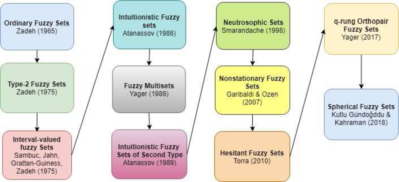
Fig. 1
Extensions of fuzzy sets.
Neutrosophic sets (NS): Smarandache (
1998) developed neutrosophic logic and neutrosophic sets (NSs) as an extension of intuitionistic fuzzy sets. The neutrosophic set is defined as the set where each element of the universe has a degree of truthfulness, indeterminacy and falsity (Liu,
2016; Ma
et al.,
2016; Liu
et al.,
2016).
Hesitant fuzzy sets (HFS): Hesitant fuzzy sets can be used as a functional tool allowing many potential degrees of membership of an element to a set. These fuzzy sets force the membership degree of an element to be possible values between zero and one (Kutlu Gundogdu
et al.,
2018; Qin
et al.,
2016; He
et al.,
2016).
Pythagorean fuzzy sets (PFS): Atanassov’s intuitionistic fuzzy sets of second type (IFS2) or Yager’s Pythagorean fuzzy sets are characterized by a membership degree and a nonmembership degree satisfying the condition that the square sum of its membership degree and nonmembership degree is equal to or less than one, which is a generalization of Intuitionistic Fuzzy Sets (IFS) (Liu
et al.,
2017; Garg,
2016; Ren
et al.,
2016; Peng and Yang,
2016).
qRung orthopair fuzzy sets (qROFs): These sets have been introduced by Yager (
2017) as an important way to express uncertain information, and they are an extension of the intuitionistic fuzzy sets and the Pythagorean fuzzy sets. Their eminent characteristic is that the sum of the qth power of the membership degree and the qth power of the degrees of non-membership is equal to or less than 1.
The spherical fuzzy sets (SFS) have been recently introduced by Kutlu Gundogdu and Kahraman (2018). SFS are based on the fundamentals of PFS and NS. The main differences between q-ROFs and SFS are the definition of hesitancy degree independently in SFS satisfying that the squared sum of membership, non-membership and hesitancy degrees is at most 1.
Pythagorean fuzzy sets (PFS) developed by Yager (
2013), which had been called Intuitionistic type-2 fuzzy sets (IFS2) by Atanassov previously (Atanassov,
1999), are characterized by a membership degree and a nonmembership degree satisfying the condition that their squared sum is at most equal to one, which is a generalization of Intuitionistic Fuzzy Sets (IFS). Hesitancy degree in PFSs calculated by
${\pi _{\tilde{p}}}=\sqrt{1-{\mu _{\tilde{p}}^{2}}(u)-{\nu _{\tilde{p}}^{2}}(u)}$.
Similar to IFSs and PFSs, neutrosophic sets (NS) are represented by the three dimensions: a truthfulness degree, an indeterminacy degree, and a falsity degree (Smarandache,
1998). NS do not only deal with the hesitancy of the system but also decrease indecisiveness of inconsistent information. Thus, the truthfulness, falsity and indeterminacy values can be independently assigned (Smarandache,
1998).
Yang and Chiclana (
2009) have proposed a new 3D spherical representation, which is called the spherical distance and allowed us to define a new distance function between intuitionistic fuzzy sets. On the surface of a sphere, the following condition is satisfied:
Let
$\tilde{A}=\{\langle u,{\mu _{\tilde{A}}}(u),{\nu _{\tilde{A}}}(u)\rangle :u\in U\}$ be an intuitionistic fuzzy set. They have
which can be equivalently transformed to
where
${x^{2}}={\mu _{\tilde{A}}}(u)$,
${y^{2}}={\nu _{\tilde{A}}}(u)$,
${z^{2}}={\pi _{\tilde{A}}}(u)$.
On a spherical surface, hesitancy can be calculated based on the given membership and non-membership values since the sum of these three parameters is exactly equal to 1 (Yang and Chiclana,
2009). Besides, they measure the spherical arc distance between two IFSs. Furthermore, Gong
et al. (
2016) introduced an approach generalizing Yang and Chiclana’s work. They applied the spherical distance measure to obtain the difference between two IFSs. They first introduced an ideal intuitionistic fuzzy estimation, and then by minimizing the spherical distance between the ideal opinion and each individual opinion in group decisions, they constructed a nonlinear optimization model.
The spherical fuzzy sets are based on the fact that the hesitancy of a decision maker can be assigned independently from membership and non-membership degrees, satisfying the following condition:
where
${\mu _{{\tilde{A}_{s}}}}:U\to [0,1]$,
${\nu _{{\tilde{A}_{s}}}}:U\to [0,1]$,
${\pi _{{\tilde{A}_{s}}}}:U\to [0,1]$ and
$0\leqslant {\mu _{{\tilde{A}_{s}}}^{2}}(u)+{\nu _{{\tilde{A}_{s}}}^{2}}(u)+{\pi _{{\tilde{A}_{s}}}^{2}}(u)\leqslant 1$,
$\forall u\in U$.
On the surface of the blue coloured sphere in Fig.
2, Eq. (
3) becomes
Since Yang and Chiclana (
2009) and Gong
et al. (
2016) only measure the arc distances on the surface of the sphere, Euclidean distance is not measured in these works. In our spherical fuzzy sets approach, the sphere is not solid but a spherical volume. Based on this fact, Euclidean distance measurement is meaningful. This also means that any two points within the spherical volume are also on the surface of another sphere; however, the sum given by Eq. (
4) becomes less than one in this case (red coloured sphere in Fig.
3). Euclidean distance gives the shortest distance between two points in the space as in Fig.
2.
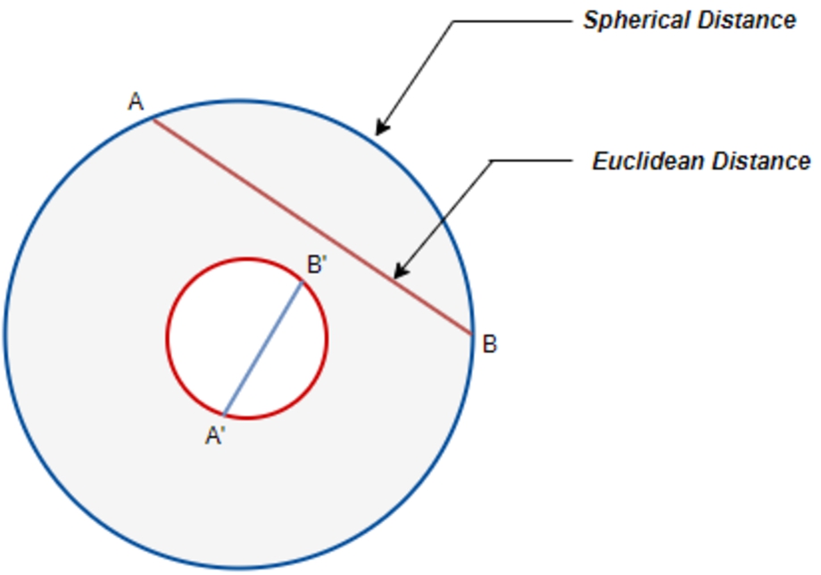
Fig. 2
Euclidean and spherical distances.
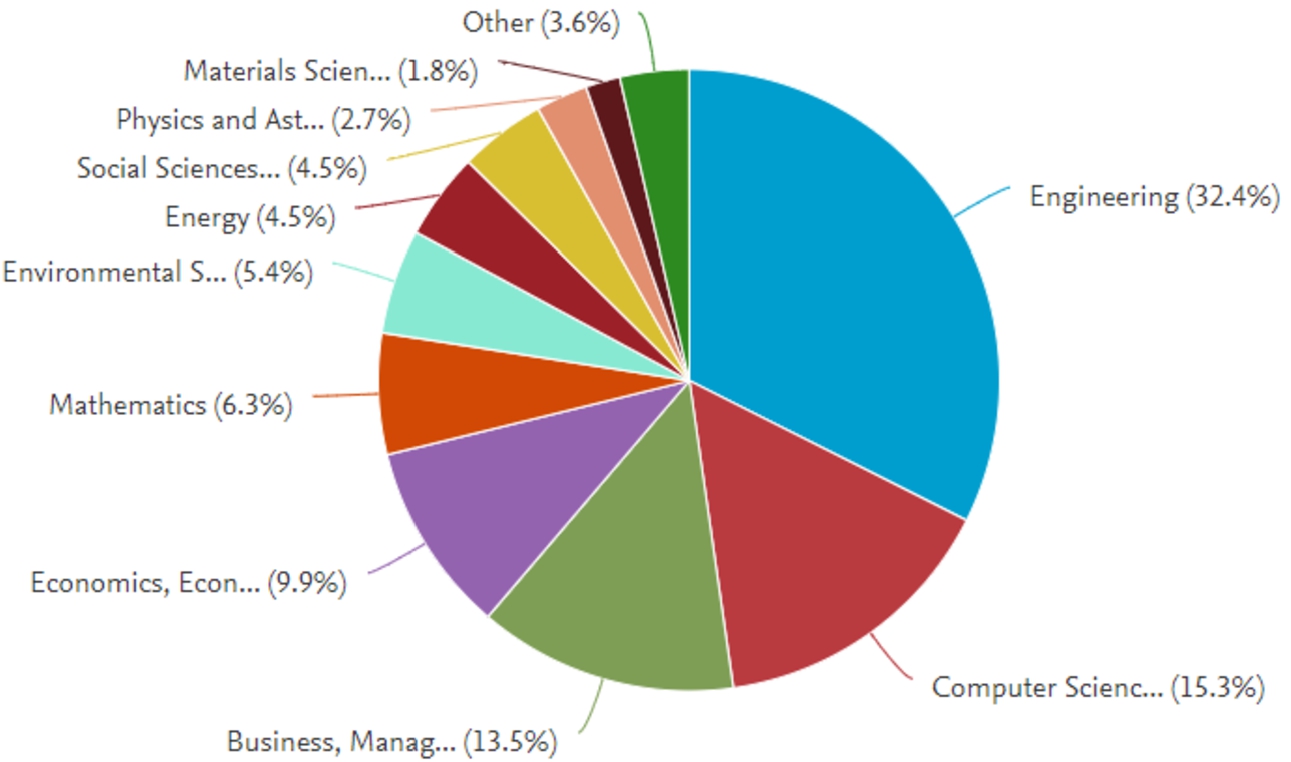
Fig. 3
Subject areas of the WASPAS papers.
In this paper, we extend one of the most used multi-criteria decision making methods, WASPAS, to its spherical fuzzy version. We illustrate its application through an industrial robot selection problem.
The rest of this paper is organized as follows. Section
2 includes the literature review on WASPAS. Section
3 gives introductory definitions on 3D fuzzy sets. In Section
4, the preliminaries on SFS are given. Section
5 includes our novel proposed MCDM method called Spherical Fuzzy WASPAS method (SF-WASPAS) and Section
6 applies SF-WASPAS method to industrial robot selection problem and also includes a comparative analysis of SF-WASPAS and IF-TOPSIS. Finally, the last section presents the conclusions and suggestions for further research.
4 Spherical Fuzzy Sets: Preliminaries
Intuitionistic and Pythagorean fuzzy membership functions are composed of membership, non-membership and hesitancy parameters, which can be calculated by
${\pi _{\tilde{I}}}=1-\mu -\nu $ or
${\pi _{\tilde{P}}}=\sqrt{1-{\mu ^{2}}-{\nu ^{2}}}$ , respectively. Neutrosophic membership functions are also defined by three parameters
truthfulness, falsity and
indeterminacy, whose sum can be between 0 and 3, and the value of each is between 0 and 1 independently. In spherical fuzzy sets, while the squared sum of membership, non-membership and hesitancy parameters can be between 0 and 1, each of them can be defined between 0 and 1 independently to satisfy that their squared sum is at most equal to 1. Figure
4 illustrates the differences among IFS, PFS, NS and SFS.
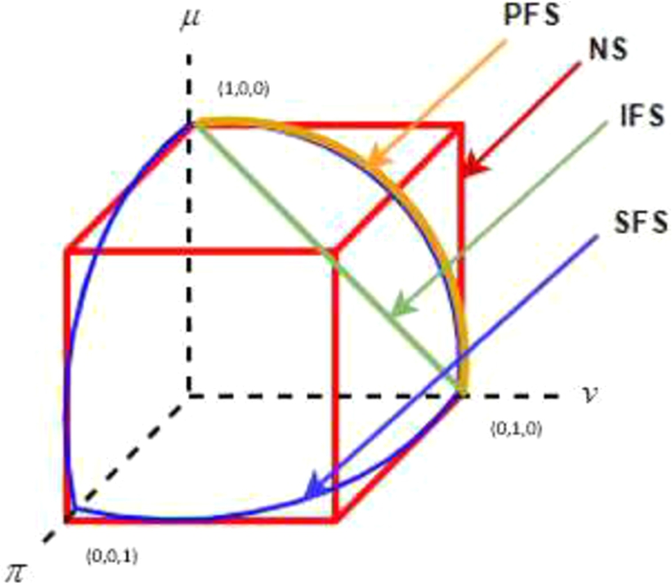
Fig. 4
Geometric representations of IFS, PFS, NS and SFS.
In this section, we give the definition of SFS and summarize spherical distance measurement, arithmetic operations, aggregation and defuzzification operations (Kutlu Gundogdu and Kahraman,
2018).
Definition 1.
Spherical Fuzzy Sets (SFS)
${\tilde{A}_{S}}$ of the universe of discourse
U is given by
where
${\mu _{{\tilde{A}_{s}}}}:U\to [0,1]$,
${\nu _{{\tilde{A}_{s}}}}:U\to [0,1]$,
${\pi _{{\tilde{A}_{s}}}}:U\to [0,1]$ and
For each
u, the numbers
${\mu _{{\tilde{A}_{s}}}}(u),{\nu _{{\tilde{A}_{s}}}}(u)$ and
${\pi _{{\tilde{A}_{s}}}}(u)$ are degree of membership, non-membership and hesitancy of
u to
${\tilde{A}_{s}}$, respectively. Geometrical representation of SFS is given in Fig.
5 (Yang and Chiclana,
2009).
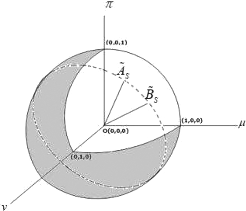
Fig. 5
Geometrical representation of spherical fuzzy sets.
Some operations are defined over the Spherical Fuzzy Sets (SFS) as below.
On the basis of relationship between SFS and PFS, we further define some novel operations for SFS as below:
Definition 2.
Basic Operators
Multiplication by a scalar: $\lambda >0$
λth power of ${\tilde{A}_{s}}$; $\lambda >0$
Definition 3.
For these SFS
${\tilde{A}_{s}}=({\mu _{{\tilde{A}_{s}}}},{\nu _{{\tilde{A}_{s}}}},{\pi _{{\tilde{A}_{s}}}})$ and
${\tilde{B}_{s}}=({\mu _{{\tilde{B}_{s}}}},{\nu _{{\tilde{B}_{s}}}},{\pi _{{\tilde{B}_{s}}}})$ , the followings are valid under the condition
$\lambda ,{\lambda _{1}},{\lambda _{2}}>0$.
Proofs of the above equations can be found in Kutlu Gundogdu and Kahraman (
2018).
Definition 4.
Spherical Weighted Arithmetic Mean (SWAM) with respect to
$w=({w_{1}},{w_{2}},\dots ,{w_{n}})$,
${w_{i}}\in [0,1]$;
${\textstyle\sum _{i=1}^{n}}{w_{i}}=1$, SWAM is defined as:
Definition 5.
Spherical Weighted Geometric Mean (SWGM) with respect to
$w=({w_{1}},{w_{2}},\dots ,{w_{n}})$,
${w_{i}}\in [0,1]$;
${\textstyle\sum _{i=1}^{n}}{w_{i}}=1$, SWGM is defined as:
Definition 6.
Score function and Accuracy function of sorting SFS are defined by
Note that:
${\tilde{A}_{s}}<{B_{s}}$ if and only if
$\mathit{Score}({\tilde{A}_{s}})<\mathit{Score}({\tilde{B}_{s}})$ or
$\mathit{Score}({\tilde{A}_{s}})=S\mathit{core}({\tilde{B}_{s}})$ and
$\mathit{Accuracy}({\tilde{A}_{s}})<\mathit{Accuracy}({\tilde{B}_{s}})$.
5 Extension of WASPAS with Spherical Fuzzy Sets
A MCDM problem can be expressed as a decision matrix whose elements indicate the evaluation values of all alternatives with respect to each criterion under Spherical fuzzy environment. Let $X=\{{x_{1}},{x_{2}},\dots ,{x_{m}}\}$ ($m\geqslant 2$) be a discrete set of m feasible alternatives and $C=\{{c_{1}},{c_{2}},\dots ,{c_{n}}\}$ be a finite set of criteria and $W=\{{w_{1}},{w_{2}},\dots ,{w_{n}}\}$ be the weight vector of all criteria which satisfies $0\leqslant {w_{j}}\leqslant 1$ and ${\textstyle\sum _{j=1}^{n}}{w_{j}}=1$.
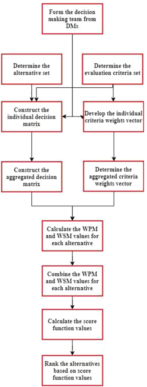
Fig. 6
SF-WASPAS proposed methodology.
The proposed spherical fuzzy WASPAS method is composed of several steps as given in this section. Before giving these steps, we present the flow chart of the SF-WASPAS method in Fig.
6 in order to make it easily understandable.
Step 1: Let DMs fill in the decision and criteria evaluation matrices using the linguistic terms given in Table
2.
Step 2: Aggregate the judgments of each decision maker (DM) using Spherical Weighted Arithmetic Mean (SWAM).
Table 2
Linguistic terms and their corresponding spherical fuzzy numbers.
|
($\mu ,\nu ,\pi $) |
| Absolutely More Importance (AMI) |
(0.9, 0.1, 0.1) |
| Very High Importance (VHI) |
(0.8, 0.2, 0.2) |
| High Importance (HI) |
(0.7, 0.3, 0.3) |
| Slightly More Importance (SMI) |
(0.6, 0.4, 0.4) |
| Equally Importance (EI) |
(0.5, 0.5, 0.5) |
| Slightly Low Importance (SLI) |
(0.4, 0.6, 0.4) |
| Low Importance (LI) |
(0.3, 0.7, 0.3) |
| Very Low Importance (VLI) |
(0.2, 0.8, 0.2) |
| Absolutely Low Importance (ALI) |
(0.1, 0.9, 0.1) |
Step 2.1: Aggregate the criteria weights. All criteria may not be assumed to be of equal importance. In order to obtain weights, all the individual decision maker opinions for the importance of each criterion need to be aggregated.
Step 2.2: Construct aggregated spherical fuzzy decision matrix based on the opinions of decision makers. Denote the evaluation values of alternative
${x_{i}}$ $(1,2,\dots ,m)$ with respect to criterion
${C_{j}}$ $(1,2,\dots ,n)$ by
${C_{j}}({\tilde{x}_{i}})=({\mu _{ij}},{\nu _{ij}},{\pi _{ij}})$ and
${\tilde{x}_{ij}}={({C_{j}}({\tilde{x}_{i}}))_{m\times n}}$ is a spherical fuzzy decision matrix. For a MCDM problem with SFS, decision matrix
${\tilde{x}_{ij}}={({C_{j}}({\tilde{x}_{i}}))_{m\times n}}$ should be constructed as in Eq. (
28).
Decision makers also evaluate the decision criteria as given in Table
3.
Table 3
Evaluation of criteria by DMs.
| Criteria |
DM1 |
DM2 |
… |
DMk |
| C1 |
$({\mu _{11}},{\nu _{11}},{\pi _{11}})$ |
$({\mu _{12}},{\nu _{12}},{\pi _{12}})$ |
… |
$({\mu _{1k}},{\nu _{1k}},{\pi _{1k}})$ |
| C2 |
$({\mu _{21}},{\nu _{21}},{\pi _{21}})$ |
$({\mu _{22}},{\nu _{22}},{\pi _{22}})$ |
… |
$({\mu _{2k}},{\nu _{2k}},{\pi _{2k}})$ |
| ⋮ |
⋮ |
⋮ |
⋱ |
⋮ |
| Cj |
$({\mu _{j1}},{\nu _{j1}},{\pi _{j1}})$ |
$({\mu _{j2}},{\nu _{j2}},{\pi _{j2}})$ |
… |
$({\mu _{jk}},{\nu _{jk}},{\pi _{jk}})$ |
Decision makers assess the alternatives with respect to the criteria as if they were benefit criteria such that they assign a lower linguistic term if it is a cost criterion.
Step 3: Calculate the score function value of each criterion in Table
3 and then normalize these values.
Step 3.1: Defuzzify the aggregated criteria weights by using the score function given in Eq. (
29).
Note that: If it is less than 0, a small number is added to all criteria weights to provide a slightly greater number than zero.
Step 3.2: Normalize the aggregated criteria weights by using Eq. (
30).
Step 4: Calculate the results of Weighted Sum Model (WSM) as presented in Eq. (
31).
Eq. (
31) can be divided into two parts for ease of operations. First, the multiplication operator, then the addition operator is performed.
Step 4.1: Calculate the multiplication part of Eq. (
31) by using Eq. (
32).
Step 4.2: Calculate each addition term in Eq. (
31) by using Eq. (
33).
Step 5: Calculate the results of Weighted Product Model (WPM) as presented in Eq. (
34).
Eq. (
34) can be also divided into two parts for ease of operations. First, the exponential operator and then the multiplication operator is performed.
Step 5.1: Calculate the exponential part of Eq. (
34) by using Eq. (
35).
Step 5.2: Calculate each multiplication term in Eq. (
34) based on Eq. (
36).
Step 6: Determine the threshold number
λ and calculate Eqs. (
37) and (
38).
Step 7: Sum Eq. (
37) and Eq. (
38) as given by Eq. (
39).
Step 8: Defuzzify by using the score function as given in Eq. (
29). We put the alternatives into order with respect to the decreasing values of score values. If the score values of two alternatives are equal, their accuracy function values might be considered as in Eq. (
26).
6 An Illustrative Example
Our proposed methodology is applied to an industrial robot selection problem. For this goal, mostly used five robots (6-axis robots X1, Scara robots X2, Dual-arm robots X3, Redundant robots X4, Cartesian robots X5) are evaluated. After a comprehensive literature review, four criteria have been determined, which are efficiency (C1), suitability (C2), automation (C3), and ergonomics (C4). The weights of three decision makers (DM1, DM2, DM3) having different experience levels are 0.4, 0.3 and 0.3, respectively.
First of all, the assessments for the criteria are collected from decision makers with respect to the goal, using the linguistic terms given in Table
2. All assessments are given in Tables
4,
5, and 6.
Table 4
Assessments of DM1.
| DM1 |
C1 |
C2 |
C3 |
C4 |
| X1 |
AMI |
SMI |
VHI |
SLI |
| X2 |
SLI |
VHI |
HI |
EI |
| X3 |
EI |
VHI |
VHI |
HI |
| X4 |
HI |
SMI |
HI |
EI |
| X5 |
HI |
HI |
LI |
SMI |
Table 5
Assessments of DM2.
| DM2 |
C1 |
C2 |
C3 |
C4 |
| X1 |
HI |
SMI |
VHI |
EI |
| X2 |
SLI |
HI |
HI |
HI |
| X3 |
SLI |
VHI |
HI |
EI |
| X4 |
SMI |
HI |
LI |
LI |
| X5 |
HI |
SMI |
HI |
SMI |
Table 6
Assessments of DM3.
| DM3 |
C1 |
C2 |
C3 |
C4 |
| X1 |
EI |
HI |
HI |
HI |
| X2 |
VHI |
EI |
EI |
EI |
| X3 |
HI |
VHI |
VHI |
HI |
| X4 |
SMI |
HI |
LI |
LI |
| X5 |
HI |
EI |
EI |
EI |
Table 7
Aggregated decision matrix.
| Alternatives |
C1 |
C2 |
C3 |
C4 |
| X1 |
(0.78, 0.23, 0.27) |
(0.63, 0.37, 0.37) |
(0.77, 0.23, 0.23) |
(0.55, 0.46, 0.40) |
| X2 |
(0.40, 0.60, 0.40) |
(0.71, 0.30, 0.32) |
(0.65, 0.35, 0.36) |
(0.58, 0.43, 0.44) |
| X3 |
(0.56, 0.45, 0.41) |
(0.80, 0.20, 0.20) |
(0.77, 0.23, 0.23) |
(0.65, 0.35, 0.36) |
| X4 |
(0.64, 0.36, 0.36) |
(0.66, 0.34, 0.34) |
(0.53, 0.50, 0.31) |
(0.40, 0.61, 0.41) |
| X5 |
(0.70, 0.30, 0.30) |
(0.62, 0.38, 0.39) |
(0.53, 0.49, 0.38) |
(0.57, 0.43, 0.43) |
Table 8
Importance weights of the criteria.
| Criteria |
DM1 |
DM2 |
DM3 |
| C1 |
AMI |
HI |
EI |
| C2 |
HI |
LI |
LI |
| C3 |
VHI |
VHI |
HI |
| C4 |
SMI |
HI |
HI |
These judgments are aggregated using SWAM operator by considering the importance levels of decision makers. Aggregated decision matrix is obtained as in Table
7.
The linguistic importance weights of the criteria assigned by DMs are shown in Table
8.
The weight of each criterion obtained by using SWAM operator is presented in Table
9.
Table 9
Aggregated criteria weights.
| Criteria |
Weight of each criterion |
| C1 |
(0.78, 0.23, 0.27) |
| C2 |
(0.53, 0.50, 0.31) |
| C3 |
(0.77, 0.23, 0.23) |
| C4 |
(0.66, 0.34, 0.34) |
After the weights of the criteria have been determined, the defuzified and normalized criteria weights are calculated by utilizing Eqs. (
33) and (
34) as given in Table
10.
Table 10
Defuzzified and normalized criteria weights.
| Criteria |
Weight of each criterion |
| C1 |
0.26681 |
| C2 |
0.00001 |
| C3 |
0.49129 |
| C4 |
0.24189 |
Based on Table
9 and Eqs. (
32) and (
33),
${\tilde{Q}_{i}^{(1)}}$ is obtained as in Table
11. Based on the first column of Table
11 and Eq. (
37),
$\lambda {\tilde{Q}_{i}^{(1)}}$ is calculated as given in the second column of Table
11.
Table 11
Weighted sum product (${\tilde{Q}_{i}^{(1)}}$).
| Alternatives |
${\tilde{Q}_{i}^{(1)}}$ |
$\lambda {\tilde{Q}_{i}^{(1)}}$ |
| X1 |
(0.75, 0.25, 0.27) |
(0.58, 0.50, 0.24) |
| X2 |
(0.57, 0.44, 0.39) |
(0.42, 0.67, 0.31) |
| X3 |
(0.69, 0.32, 0.32) |
(0.53, 0.56, 0.27) |
| X4 |
(0.57, 0.45, 0.35) |
(0.42, 0.67, 0.28) |
| X5 |
(0.62, 0.39, 0.36) |
(0.46, 0.63, 0.29) |
According to Table
10 and Eqs. (
35) and (
36),
${\tilde{Q}_{i}^{(2)}}$ is obtained as in Table
12. Based on the first column of Table
12 and Eq. (
38),
$(1-\lambda ){\tilde{Q}_{i}^{(2)}}$ is calculated as given in the second column of Table
12.
Table 12
Weighted product model (${\tilde{Q}_{i}^{(2)}}$).
| Alternatives |
${\tilde{Q}_{i}^{(2)}}$ |
$(1-\lambda ){\tilde{Q}_{i}^{(2)}}$ |
| X1 |
(0.74, 0.28, 0.29) |
(0.57, 0.53, 0.25) |
| X2 |
(0.53, 0.48, 0.39) |
(0.39, 0.69, 0.31) |
| X3 |
(0.66, 0.35, 0.34) |
(0.50, 0.59, 0.29) |
| X4 |
(0.55, 0.47, 0.35) |
(0.40, 0.69, 0.28) |
| X5 |
(0.60, 0.42, 0.36) |
(0.45, 0.65, 0.30) |
In the next step, based on Tables
11 and
12, we can calculate the final value of SF-WASPAS using Eq. (
39). They are given in Table
13.
Table 13
${\tilde{Q}_{i}}$ values.
| Alternatives |
${\tilde{Q}_{i}}$ |
| X1 |
(0.744, 0.268, 0.279) |
| X2 |
(0.548, 0.463, 0.392) |
| X3 |
(0.677, 0.335, 0.331) |
| X4 |
(0.558, 0.460, 0.350) |
| X5 |
(0.607, 0.406, 0.360) |
From Table
13, the score value of each alternative is calculated based on Eq. (
29) and given in Table
14.
Table 14
Score values and ranking.
| Alternatives |
Score |
Ranking |
| X1 |
0.217 |
1 |
| X2 |
0.019 |
5 |
| X3 |
0.120 |
2 |
| X4 |
0.031 |
4 |
| X5 |
0.059 |
3 |
The score values indicate that the best alternative is X1 and overall ranking is $X1>X3>X5>X4>X2$.
7 Comparative and Sensitivity Analyses
We compare the proposed SF-WASPAS with intuitionistic fuzzy TOPSIS (IF-TOPSIS) in this section. Table
15 presents the IF linguistic scale, which we use for comparison purposes.
Table 15
IF linguistic scale (Boran
et al.,
2009).
| Linguistic terms |
$(\mu ,\nu ,\pi )$ |
| Absolutely more Importance (AMI) |
(0.9, 0.1, 0) |
| Very High Importance (VHI) |
(0.8, 0.1, 0.1) |
| High Importance (HI) |
(0.7, 0.2, 0.1) |
| Slightly More Importance (SMI) |
(0.6, 0.3, 0.1) |
| Equally Importance (EI) |
(0.5, 0.4, 0.1) |
| Slightly Low Importance (SLI) |
(0.4, 0.5, 0.1) |
| Low Importance (LI) |
(0.25, 0.6, 0.15) |
| Very Low Importance (VLI) |
(0.1, 0.75, 0.15) |
| Absolutely Low Importance (ALI) |
(0.1, 0.9, 0) |
In this comparison, the same judgments as given in Tables
4,
5 and
6 were used and aggregated using IFWA (Intuitionistic Fuzzy Weighted Average) operator given in Eq. (
40) (Xu,
2007). Aggregated decision matrix is given in Table
16.
Table 16
Aggregated decision matrix.
| Alternatives |
C1 |
C2 |
C3 |
C4 |
| X1 |
(0.77, 0.19, 0.04) |
(0.70, 0.20, 0.10) |
(0.81, 0.15, 0.03) |
(0.80, 0.17, 0.03) |
| X2 |
(0.57, 0.31, 0.12) |
(0.72, 0.20, 0.08) |
(0.73, 0.16, 0.11) |
(0.45, 0.45, 0.10) |
| X3 |
(0.55, 0.35, 0.11) |
(0.49, 0.39, 0.12) |
(0.73, 0.16, 0.11) |
(0.45, 0.42, 0.13) |
| X4 |
(0.64, 0.26, 0.10) |
(0.61, 0.28, 0.12) |
(0.61, 0.24, 0.14) |
(0.61, 0.28, 0.11) |
| X5 |
(0.70, 0.20, 0.10) |
(0.62, 0.28, 0.10) |
(0.50, 0.38, 0.12) |
(0.57, 0.33, 0.10) |
The same criteria judgments given in Table
8 are used for this comparison. Opinions of decision makers on criteria are aggregated using IFWA operator and the weight of each criterion is presented in Table
17.
Table 17
Aggregated criteria matrix.
| Criteria |
Weight of each criterion |
| C1 |
(0.77, 0.19, 0.04) |
| C2 |
(0.48, 0.39, 0.13) |
| C3 |
(0.77, 0.12, 0.10) |
| C4 |
(0.66, 0.24, 0.10) |
After the weights of the criteria and the rating of the alternatives have been determined, the aggregated weighted intuitionistic fuzzy decision matrices are constructed by utilizing Eqs. (
41) and (
42) as given in Table
18.
and
Table 18
Aggregated weighted decision matrix.
| Alternatives |
C1 |
C2 |
C3 |
C4 |
| X1 |
(0.60, 0.34, 0.06) |
(0.30, 0.55, 0.15) |
(0.60, 0.23, 0.17) |
(0.36, 0.51, 0.14) |
| X2 |
(0.44, 0.44, 0.12) |
(0.34, 0.50, 0.16) |
(0.50, 0.34, 0.16) |
(0.38, 0.48, 0.14) |
| X3 |
(0.42, 0.47, 0.11) |
(0.38, 0.45, 0.17) |
(0.60, 0.23, 0.17) |
(0.43, 0.42, 0.15) |
| X4 |
(0.50, 0.39, 0.11) |
(0.32, 0.53, 0.15) |
(0.37, 0.46, 0.17) |
(0.24, 0.63, 0.13) |
| X4 |
(0.54, 0.35, 0.11) |
(0.30, 0.56, 0.15) |
(0.38, 0.46, 0.16) |
(0.38, 0.49, 0.13) |
Positive and negative ideal solutions are given in Table
19. They are calculated by using Eqs. (
43) and (
44).
Table 19
Positive and negative ideal solutions.
|
C1 |
C2 |
C3 |
C4 |
| X*(Best) |
(0.60, 0.34, 0.06) |
(0.38, 0.45, 0.17) |
(0.60, 0.23, 0.17) |
(0.43, 0.42, 0.15) |
| X-(Worst) |
(0.42, 0.47, 0.11) |
(0.30, 0.55, 0.15) |
(0.37, 0.46, 0.17) |
(0.24, 0.63, 0.13) |
Based on Eq. (
45), we can calculate the Euclidean distances between alternative
${X_{i}}$ and SF-PIS as well as
${X_{i}}$ and SF-NIS. They are given in Table
20 (Szmidt and Kacprzyk,
2000).
Table 20
Distances to positive and negative ideal solutions.
| Alternatives |
${D_{E}}({X_{i}},{X^{\ast }})$ |
${D_{E}}({X_{i}},{X^{-}})$ |
| X1 |
0.061 |
0.151 |
| X2 |
0.095 |
0.098 |
| X3 |
0.079 |
0.158 |
| X4 |
0.162 |
0.038 |
| X5 |
0.128 |
0.092 |
Closeness ratios are calculated based on Eq. (
46) and presented in Table
21.
Table 21
Closeness ratio of each alternative.
| Alternatives |
Closeness ratio |
Ranking |
| X1 |
0.713 |
1 |
| X2 |
0.509 |
3 |
| X3 |
0.666 |
2 |
| X4 |
0.192 |
5 |
| X5 |
0.419 |
4 |
Table 22
Rankingof the alternatives.
| Alternatives |
IF-TOPSIS |
SF-WASPAS |
| X1 |
1 |
1 |
| X2 |
5 |
3 |
| X3 |
2 |
2 |
| X4 |
4 |
5 |
| X5 |
3 |
4 |
The closeness ratios based on IF-TOPSIS method indicate that the best alternative is X1 and the overall ranking is
$X1>X3>X2>X5>X4$. Table
22 presents the ranking of the alternatives according to the IF-TOPSIS and SF-WASPAS methods. We can say that the first alternative should be selected among the industrial robot alternatives.
We applied a sensitivity analysis by changing the threshold number
λ and observed the robustness of the given decisions. Sensitivity analysis showed that very robust decisions have been obtained from SF-WASPAS as given in Fig.
7. Although the appraisal scores changed, the ranking of alternatives remained the same.
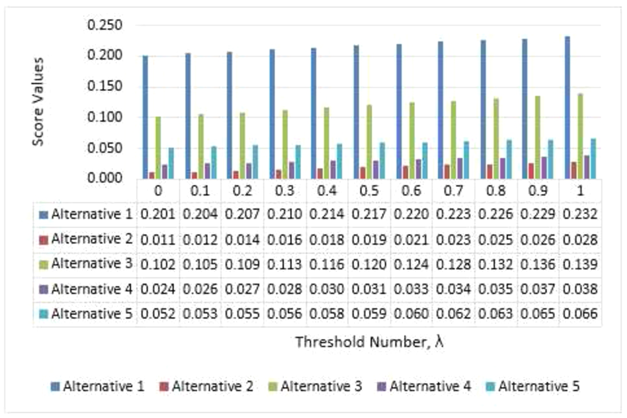
Fig. 7
Sensitivity analysis by changing threshold value, λ.
8 Conclusion and Future Work
Three dimensional membership functions have been very popular in the recent years. IFS, PFS, and NS use those kinds of membership functions. Spherical fuzzy sets are an attempt to provide a general view to three dimensional fuzzy sets. We presented the theory of spherical fuzzy sets (SFS) and their arithmetic operations in this paper together with their aggregation operators. This new type of fuzzy sets has been used in the extension of WASPAS to SF-WASPAS, which is a weighted combination of WSM and WPM methods. In SF-WASPAS, spherical fuzzy sets have been used in all of the steps without making any defuzzification, except the calculation of the weights of the criteria. Through the proposed SF-WASPAS, DMs could assign their judgments on the membership, non-membership and hesitancy degrees as independent parameters under spherical fuzzy uncertainty environment.
An industrial robot selection problem has been successfully solved by SF-WASPAS and compared with IF-TOPSIS. Comparative analysis with IF-TOPSIS showed the validity of the obtained results by SF-WASPAS with slight changes. Additionally, we applied a sensitivity analysis by changing threshold value (λ) and observed the robustness of the given decisions. Sensitivity analysis showed that very robust decisions have been obtained from SF-WASPAS.
For further research, we suggest SF-WASPAS to be compared with other extensions of MCDM methods such as SF-CODAS, SF-TOPSIS, SF-AHP and SF-VIKOR.

