Informatica logo


Login Register

  1. Home
  2. Issues
  3. Volume 28, Issue 3 (2017)
  4. Self-Adaptive and Adaptive Parameter Con ...

Informatica

Information Submit your article For Referees Help ATTENTION!
  • Article info
  • Full article
  • Related articles
  • Cited by
  • More
    Article info Full article Related articles Cited by

Self-Adaptive and Adaptive Parameter Control in Improved Artificial Bee Colony Algorithm
Volume 28, Issue 3 (2017), pp. 415–438
Bekir Afşar   Doğan Aydin   Aybars Uğur   Serdar Korukoğlu  

Authors

 
Placeholder
https://doi.org/10.15388/Informatica.2017.136
Pub. online: 1 January 2017      Type: Research Article      Open accessOpen Access

Received
1 June 2015
Accepted
1 September 2016
Published
1 January 2017

Abstract

The Improved Artificial Bee Colony (IABC) algorithm is a variant of the well-known Artificial Bee Colony (ABC) algorithm. In IABC, a new initialization approach and a new search mechanism were added to the ABC for avoiding local optimums and a better convergence speed. New parameters were added for the new search mechanism. Specified values of these newly added parameters have a direct impact on the performance of the IABC algorithm. For better performance of the algorithm, parameter values should be subjected to change from problem to problem and also need to be updated during the run of the algorithm. In this paper, two novel parameter control methods and related algorithms have been developed in order to increase the performance of the IABC algorithm for large scale optimization problems. One of them is an adaptive parameter control which updates parameter values according to the feedback coming from the search process during the run of the algorithm. In the second method, the management of the parameter values is left to the algorithm itself, which is called self-adaptive parameter control. The adaptive IABC algorithms were examined and compared to other ABC variants and state-of-the-art algorithms on a benchmark functions suite. Through the analysis of the results of the experiments, the adaptive IABC algorithms outperformed almost all ABC variants and gave competitive results with state-of-the-art algorithms from the literature.

1 Introduction

Swarm intelligence (SI) is a research area that aims at understanding on the self-organized swarms. An ant colony, a flock of birds and a school of fish are typical examples of swarm intelligence. These swarms have to overcome some problems during their lives such as liaising, foraging, orientation to the right direction, etc. Researchers were inspired by problem-solving skills and behaviours of swarms and proposed new algorithms for numerical optimization problems. For instance, particle swarm optimization (PSO) was inspired from the behaviours of bird flocking or fish schooling (Kennedy, 2010), ant colony optimization (ACO) was inspired from foraging behaviour of ant colonies (Dorigo, 1992), and cuckoo search algorithm (CS) was inspired from the behaviours of cuckoos during their incubation period (Yang and Deb, 2010). These are swarm intelligence based algorithms.
Swarm intelligence algorithms are the metaheuristics that are developed independently of the optimization problems. These algorithms have some critical parameters that should be tuned carefully according to the tackling problem instance. Therefore, parameter tuning is a key research area for the optimization algorithms to show similar good performances on the different optimization problems. In literature, there are many studies on parameter adaptation for metaheuristics. The several instances of parameter adaptation methods can be found on Evolutionary Algorithms (Eiben et al., 1999; Lobo et al., 2007), Differential Evolution (Abbass, 2002; Das and Suganthan, 2011; Gämperle et al., 2002; Qin et al., 2009; Ronkkonen et al., 2005), Ant Colony Optimization (Zhaoquan et al., 2009; Hao et al., 2007; Stützle et al., 2012) and so on.
Artificial Bee Colony (ABC) algorithm (Karaboga and Basturk, 2007) is another swarm intelligence based optimization algorithm, inspired from foraging behaviours of honey bees. ABC was applied to continuous optimization problems successfully, although it has some deficiencies. ABC has few parameters which are not very sensitive to the problem type. However, in recent years, several variants of ABC algorithm, which come with additional tunable parameters, have been proposed to enhance search ability and to increase convergence speed to achieve global optimum.
Improved ABC (IABC) algorithm (Gao and Liu, 2011) is a recent variant of ABC algorithm which proposes a new initialization strategy and a probabilistic search mechanism to improve solution quality. IABC has significant results with the other ABC variants on the low dimensional problems but the performance of IABC decreases dramatically when the dimension of the problem increases (Liao et al., 2013). IABC comes with two new tunable parameters that are very sensitive to given problem. These parameters should be set carefully for each problem, otherwise it leads to the algorithm producing good outcome in some problems, while bad results are produced with some other problems. To overcome this problem, adaptive parameter selection is needed as in other metaheuristic algorithms.
For this purpose, two different adaptive parameter selection mechanisms, that are based on self-adaptive and adaptive parameter control strategies, are proposed in this paper. With the proposed mechanisms, appropriate values of the parameters are tried to be found with feedback from the search process and they are updated online if necessary. As a result, IABC can achieve good results not only for low-dimensional but also high-dimensional problems.
This paper is structured as follows. In Section 2 we will first give details of the original ABC and IABC algorithms. Section 3 addresses two different proposed adaptive IABC algorithms under this study. Section 4 points out experimental results which include the comparisons of the proposed algorithm to IABC, other ABC variants and state-of-the-art algorithms. Section 5 concludes the article.

2 Background

In this paper, we proposed two different parameter control mechanisms in order to enhance performance of the IABC algorithm on the high-dimensional optimization problems. In the following subsections, brief descriptions of the ABC and IABC algorithms are given.

2.1 Original Artificial Bee Colony (ABC) Algorithm

In ABC algorithm (given in Algorithm 1), there are three types of honey bees as employed, onlooker and scout. The employed bees are responsible for calculating the nectar amount of every possible food sources. The number of the employed bees in the population is equal to the number of food sources in the feeding area. The onlookers are charged with choosing the food source which has a great amount of nectar. The number of the onlookers in the population is equal to the number of employed bees. The scouts are responsible for discovering new food sources. If a food source is exhausted, the employed bee becomes onlooker and the new food source discovered by the scout bee replaces the old food source.
info1156_g001.jpg
Algorithm 1
Artificial Bee Colony Algorithm.
Position of the food source represents the possible solution of the optimization problem aimed to be solved. High nectar amount of the food source means that the possible solution of the optimization problem is good. Therefore, quality of the possible solution is represented by the nectar amount and this value is called fitness value in ABC algorithm. At initialization step, $\mathit{SN}$ (number of food sources) is established randomly by using the Eq. (1):
(1)
\[ {x_{i,j}}={x_{j}^{\min }}+{\varphi _{i,j}}\big({x_{j}^{\max }}-{x_{j}^{\min }}\big)\]
where ${\varphi _{i,j}}$ is a uniform random number in $[0,1]$, ${x_{j}^{\min }}$ is the minimum value of the jth dimension while ${x_{j}^{\max }}$ is the maximum value of that dimension. Moreover, each solution (or each food source) has a fitness and limit value. limit value is used to control whether the food source has been exhausted or not.
In ABC algorithm, fitness value is calculated in accordance with the Eq. (2):
(2)
\[ {\mathit{fitness}_{i}}=\left\{\begin{array}{l@{\hskip4.0pt}l}\frac{1}{1+{f_{i}}},\hspace{1em}& {f_{i}}\geqslant 0,\\ {} 1+abs({f_{i}}),\hspace{1em}& {f_{i}}<0\end{array}\right.\]
where ${f_{i}}$ is the objective value of ith solution.
Following the initialization stage, employed bees try to find the new candidate solution based on the Eq. (3):
(3)
\[ {v_{i,j}}={x_{i,j}}+{\varphi _{i,j}}({x_{i,j}}-{x_{k,j}}),\hspace{1em}i\ne k\]
where ${v_{i,j}}$ represents the new solution to be found, ${x_{i,j}}$ is the previous solution, ${\varphi _{i,j}}$ is the random number between the range of $[-1,1]$, and ${x_{k,j}}$ is the neighbouring solution. k is rated between 1 and $SN$, while j is rated between 1 and D (maximum number of dimensions). If the candidate solution found is better than the previous one, then it supersedes. Later on, like employed bees, onlooker bees also try to find new good food sources. However, in selecting food sources, onlooker bees as different from the employed bees prefer the ones above a certain probability value ${p_{i}}$. This probability value can be seen in the Eq. (4):
(4)
\[ {p_{i}}=\frac{f{\mathit{itness}_{i}}}{{\textstyle\textstyle\sum _{n=1}^{\mathit{SN}}}{\mathit{fitness}_{n}}}.\]
Observing the behaviour of employed and onlooker bees, it is evident that they search for good food sources and focus on good solutions. Algorithm should explore new solutions to avoid local optimums. If employed and onlooker bees cannot improve a food source for limit times, it means exhaustion of that food source. Exhausted food resource is a source that is not good enough to produce new solutions. In ABC algorithm, scout bees are responsible for the exploration of new solutions searched to avoid local optimums, and they explore new food sources by utilizing the Eq. (1) instead of exhausted food sources.
However, it is seen that in certain problems, convergence speed of ABC algorithm is slow in comparison with the other population based algorithms and sticks to local optimums. Thus, new ABC algorithm versions have been proposed to increase its convergence speed.

2.2 Improved Artificial Bee Colony (IABC) Algorithm

In IABC algorithm, Gao and Liu (2011) proposed some modifications on the steps of original ABC algorithm. The first is an efficient initialization strategy that leads algorithm to find good initial population. Instead of the initialization with normal distribution in original ABC, the initialization approach of IABC utilizes chaotic systems and opposition-based learning. In detail, a chaotic random generator is used to create initial solutions. Then, the initial solutions are duplicated by opposition-based initialization. Finally, the initial population is obtained by selecting the best solutions. The procedure of this initialization strategy is given in Algorithm 2.
info1156_g002.jpg
Algorithm 2
Initialization step of IABC algorithm (Gao and Liu, 2011).
In search equations of the employed and onlooker bees steps, IABC offered two modifications as well. Contrary to original ABC, IABC emphasizes in controlling the number of decision variables changed in search equation by adding a new parameter called m. Second modification in search mechanism is that IABC comes with a probabilistic selection of two search equations, called as “ABC/best/1” (Eq. (5)) and “ABC/rand/1” (Eq. (6)) (Gao and Liu, 2011).
(5)
\[ {v_{i,m}}={x_{\mathit{best},m}}+{\varphi _{i,j}}({x_{i,m}}-{x_{r1,m}}),\]
(6)
\[ {v_{i,m}}={x_{r1,m}}+{\varphi _{i,j}}({x_{i,m}}-{x_{r2,m}})\]
where m parameter is used to control how many dimensions will be updated. ${x_{\mathit{best},m}}$ represents the best solution till then. ${x_{r1,m}}$ and ${x_{r2,m}}$ represent the randomly selected solutions. While “ABC/best/1” is used to produce new solutions based on the information of the best-so-far solutions “ABC/rand/1” is used to search the whole population. Moreover, “ABC/best/1” ensures the finding of the optimum solution quickly, while “ABC/rand/1” enables the avoidance from local optimums. Utilizing these two equations together leads to an increase in the convergence speed towards global optimum and helps to avoid local optimums. By this it means, it has been aimed to balance exploration and exploitation abilities of IABC. The probabilistic selection of these two search equations is controlled by p ($0\leqslant p\leqslant 1$) parameter. The procedure of this new searching strategy is given in Algorithm 3.
info1156_g003.jpg
Algorithm 3
Searching new solutions in IABC algorithm (Gao and Liu, 2011).
The additional parameters of IABC, m and p, have direct effect on IABC performance. Therefore, authors of IABC tried to find out appropriate values of these parameters from one problem to another. Therefore, with the appropriate parameter values, IABC shows good performance on low-dimensional benchmark functions. However, Liao et al. (2013) have detected that its performance worsens in high dimensional problems. The reason of producing good results in low dimensional problems while putting forward bad results in high dimensional problems is that the value of m and p parameters used in the proposed search mechanisms do not change depending on the problem. The m parameter shows the number of parameters to be updated in a repeat cycle in employed and onlooker bee stages. The effect of m parameter on performance is seen directly in line with the increase in the dimension of the problem.

3 The Proposed Adaptive IABC Algorithms

In this paper, we developed two new adaptive IABC versions. The first is adaptive improved ABC that uses adaptive parameter control and the second is self-adaptive improved ABC that uses self-adaptive parameter control. In adaptive parameter control, strategic parameter values are updated based on the behaviour of the algorithm in the running phase, namely feedbacks from the searching process. On the other hand, in self-adaptive parameter control, the strategic parameters become a part of solution array and thus mutate. Appropriate parameter values help to have good solutions and ensure that good candidate solutions are selected; thus these appropriate parameter values can be handed down to the forthcoming population (Eiben et al., 1999). Hence, it is different from adaptive parameter control. Parameters are involved in evolutionary progress and their values are tried to be improved.

3.1 Adaptive IABC (AIABC) Algorithm

AIABC tries to increase performance by making online updates for m and p strategic parameters having a direct effect on the performance of IABC through adaptive parameter control. In adaptive parameter control, strategic parameters are updated according to the feedbacks to be obtained in the search process during the performance of the algorithm. With this approach, the algorithm will become adaptive to the problem and it will be ensured that it displays good performance in high dimensional optimization problems.
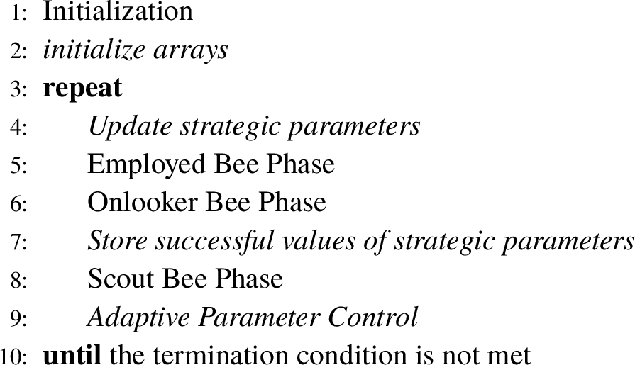
In this version, randomly generated candidate values of m and p parameters are kept in two separate arrays (mArray and pArray). In onlooker bee stage, the values in the array are used in turn for m and p parameters. If the best solution found so far has changed by using m and p values, these successful m and p values are kept in two separate arrays (sMarray and sParray). Figure 1 shows the relations of these four arrays. When all candidate values in sMarray and sParray are used, re-initialization of these arrays is made by using random values beside the ones in sMarray and sParray. By this it means, it is aimed to achieve good parameter values through the utilization of successful experiences in different stages of the problem during the performance of the algorithm. The pseudo-code of AIABC can be seen in Algorithm 4. The proposed modifications are presented in italic form in the Algorithm 4.
info1156_g004.jpg
Fig. 1
Re-generation and re-initialization of arrays holding the values of m and p parameters in AIABC algorithm.
info1156_g005.jpg
Algorithm 4
The Adaptive Improved ABC (AIABC) Algorithm.
The method developed to update the online values of m and p parameters is realized through the determination of new values by utilizing previous successful experiences during the performance of the algorithm. There are arrays including the possible ranges for each parameter (mArray for m and pArray for p).
\[\begin{array}{l}\displaystyle {\mathit{mArray}_{i}}=\big({m_{i}^{1}},{m_{i}^{2}},\dots ,{m_{i}^{\mathit{maxCount}}}\big),\hspace{1em}{m_{i}^{j}}\in [1,2],\\ {} \displaystyle {\mathit{pArray}_{i}}=\big({p_{i}^{1}},{p_{i}^{2}},\dots ,{p_{i}^{\mathit{maxCount}}}\big),\hspace{1em}{p_{i}^{j}}\in [0,1].\end{array}\]
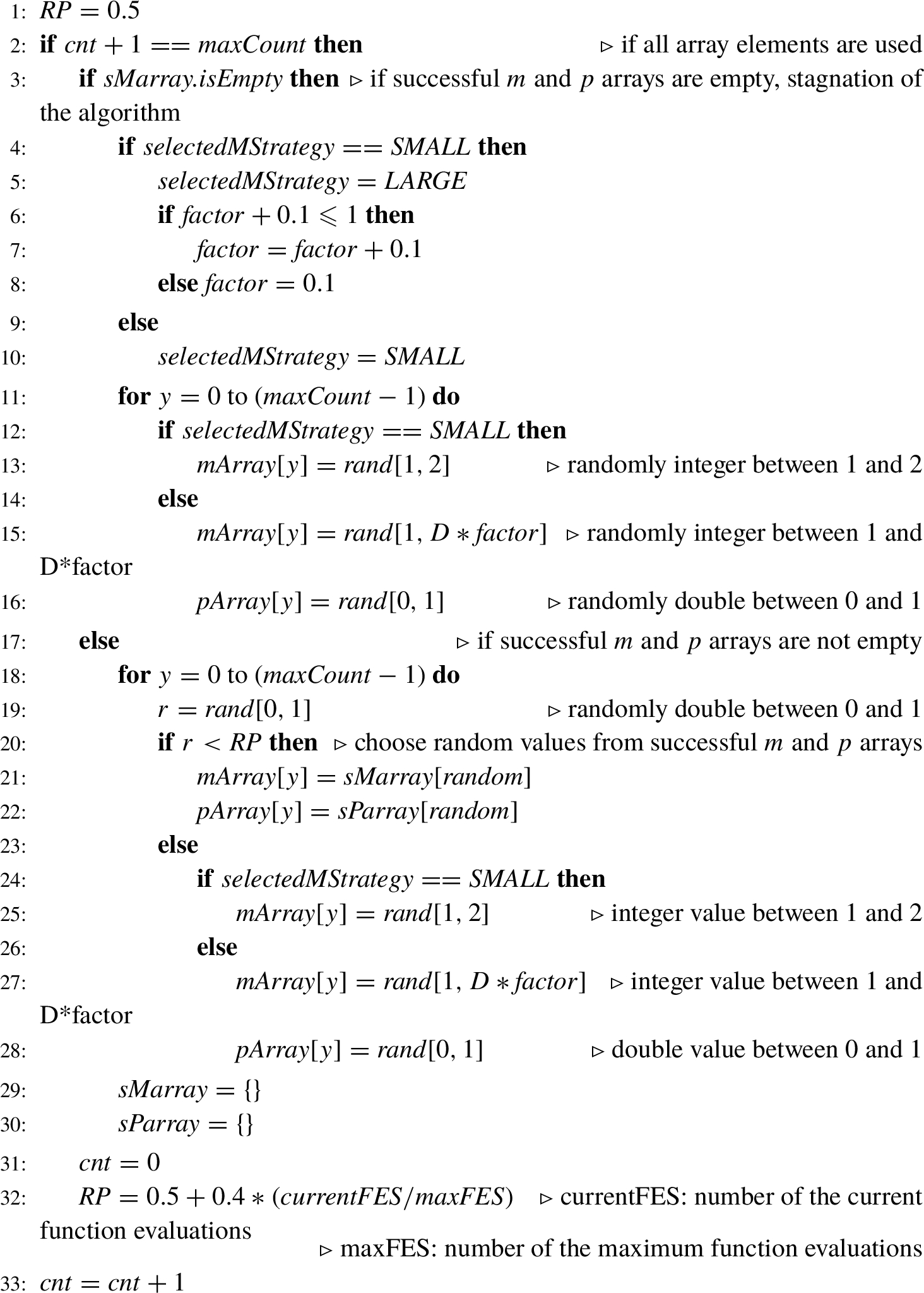
Each array includes values as many as maxCount. The process begins with $\mathit{cnt}=1$, which is used as a counter. Before each employed bee stage, values are determined as $m={m_{i}^{\mathit{cnt}}}$, $p={p_{i}^{\mathit{cnt}}}$. In employed bee stage, the algorithm continues its performance with these values. If the best-so-far solution is improved further, m and p values used in that cycle are transferred to ${\mathit{sMarray}_{i}}$ and ${\mathit{sParray}_{i}}$. When cnt counter reaches to maxCount value representing the size of arrays, re-initialization process is started for mArray and pArray. In the re-initialization process, mArray and pArray are updated by taking values randomly selected within the adaptively adjusted ranges or by taking from a certain number of successful values in ${\mathit{sMarray}_{i}}$ and ${\mathit{sParray}_{i}}$. The selection mechanism is controlled randomly by using re-initialization probability value (RP). RP is increased gradually in the running of algorithm and thus, successful m and p values can be selected more than random values in later iterations. Moreover, when all the elements of mArray and pArray are used but successful arrays are still empty, the stagnation is detected. This time, mArray and pArray are re-initialized with new random values by utilizing the ranges of parameters adaptively.
info1156_g006.jpg
Algorithm 5
Adaptive Parameter Control Procedure in AIABC Algorithm.
Determination of the possible range of m parameter properly will also have a positive effect on the performance of the algorithm. For instance, it is detected that the high values for m may have a negative effect on the performance of the algorithm specifically for high dimensional functions (Liao et al., 2013; Aydın, 2015). Therefore, the range of these parameters is adjusted adaptively while algorithm is running.
In the first random initialization, the range of m is kept $[1,2]$. In the following initializations, an adaptive approach is applied in the determination of the range of m parameter. If all elements of mArray and pArray are used and any of them is not transferred to sMarray and sParray in onlooker bee stage and the stagnation is detected, range of m parameter is changed. If the range of m is between 1 and $D\ast \mathit{factor}$ ($\mathit{LARGE}$ strategy), it is changed to between 1 and 2 ($\mathit{SMALL}$ strategy). On the contrary, when the range of m is between 1 and 2, it is changed to 1 and $D\ast \mathit{factor}$ after stagnation. The initial value of $\mathit{factor}$ variable is 0.1 and is increased by 0.1 after each stagnation. When this variable reaches 1, it is then reduced to 0.1 again. In other words, the maximum value of m is 10% of the problem dimension in the first stage; it is increased by 10% after each stagnation. When range of m parameter reaches to problem dimension, it is then reduced to 10% of the problem dimension again. Moreover, in each stagnation of the algorithm, $\mathit{mArray}$ and $\mathit{pArray}$ are re-initialized according to the range determined above. So, values leading to stagnation are changed. The whole process of adaptive parameter control procedure mentioned here is presented in Algorithm 5.

3.2 Self-Adaptive IABC (SaIABC) Algorithm

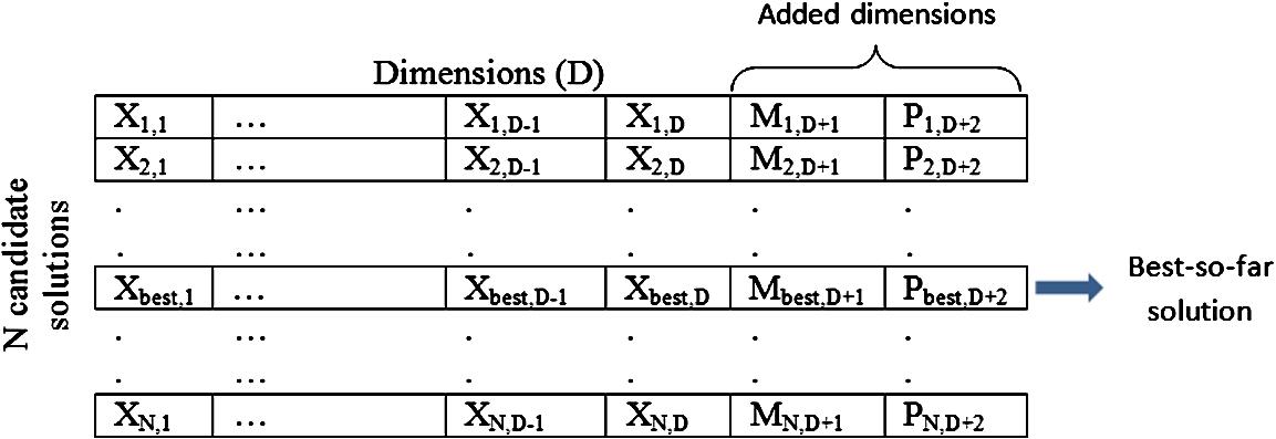
In the self-adaptive parameter control (Eiben et al., 1999), parameters to be controlled are encoded to solution chromosome as gene in evolutionary algorithms while they are encoded as a new dimension to the solution vector in SaIABC (Fig. 2). m and p parameters are added to each candidate solution as two new dimensions. If in the employed and onlooker bee search equations, these dimension values can be modified just as the dimensions of the problem and m and p values can be changed. Therefore, the control of these parameters depends on the algorithm itself.
info1156_g007.jpg
Fig. 2
New structure of solution arrays in SaIABC algorithm.
SaIABC algorithm uses values found in two additional dimensions of the best-so-far solution as m and p values for each iteration. Search equations in employed and onlooker bee stages are performed according to these parameter values. The range of m parameter is as well adjusted adaptively as in AIABC. The only difference is determination of algorithm stagnation. Here, if the algorithm cannot improve the best-so-far solution at some consecutive iterations (i.e. 25 iterations), this means algorithm stagnates and changes the strategy from LARGE to SMALL or vice versa.

4 Experimental Results

In this section, three different comparisons are explained in order to show the proposed adaptive IABCs are competitive with other algorithms. In the first experiment, we compared adaptive IABCs and the other ABC variants with default parameter values. In second, we did the same comparison with tuned parameter values. Also some statistical tests are presented to show the statistical difference. The adaptive IABCs are compared with the state-of-the-art algorithms in the third experiment.

4.1 Experimental Setup

In this section, the proposed adaptive IABC algorithms are applied to minimize a set of 19 scalable functions presented by Lozano et al. (2011) for Soft Computing (SOCO) special issue. Some of them $({f_{1}},{f_{2}},{f_{7}},{f_{8}},{f_{9}},{f_{10}},{f_{11}})$ are unimodal and the others are multimodal functions. These benchmark functions and their peculiarities are described in Table 1.
Table 1
The benchmark functions (Lozano et al., 2011).
Name Definition Range Uni./Multi. Separable
${f_{1}}$: Shifted sphere function ${\textstyle\sum _{i=0}^{n}}{z_{i}^{n}}$ ${[-100,100]^{n}}$ U yes
${f_{2}}$: Shifted Schwefelś problem 2.21 ${\max _{i}}\{|{z_{i}},1\leqslant i\leqslant n|\}$ ${[-100,100]^{n}}$ U no
${f_{3}}$: Shifted Rosenbrockś function ${\textstyle\sum _{i=1}^{n-1}}[100{({z_{i}^{2}}-{z_{i}}+1)^{2}}+{({z_{i}}-1)^{2}}]$ ${[-100,100]^{n}}$ M no
${f_{4}}$: Shifted Rastriginś function $10n+{\textstyle\sum _{i=1}^{n}}({z_{i}^{2}}-10\cos (2\pi {z_{i}}))$ ${[-5,5]^{n}}$ M yes
${f_{5}}$: Shifted Griewankś function $\frac{1}{1000}{\textstyle\sum _{i=1}^{n}}{z_{i}^{2}}-{\textstyle\prod _{i=1}^{n}}\cos (\frac{{z_{i}}}{\sqrt{i}})+1$ ${[-600,600]^{n}}$ M no
${f_{6}}$: Shifted Ackleyś function $-20{e^{-0.2\sqrt{\frac{1}{n}{\textstyle\sum _{i=1}^{n}}{z_{i}^{2}}}}}-{e^{\frac{1}{n}{\textstyle\sum _{i=1}^{n}}\cos (2\pi {z_{i}})}}+20+e$ ${[-32,32]^{n}}$ M yes
${f_{7}}$: Shifted Schwefelś problem 2.22 ${\textstyle\sum _{i=1}^{n}}|{z_{i}}|+{\textstyle\prod _{i=1}^{n}}|{z_{i}}|$ ${[-10,10]^{n}}$ U yes
${f_{8}}$: Shifted Schwefelś problem 1.2 ${\textstyle\sum _{i=1}^{n}}{({\textstyle\sum _{j=1}^{i}}{z_{j}})^{2}}$ ${[-65.536,65.536]^{n}}$ U no
${f_{9}}$: Shifted extended f10 ${\textstyle\sum _{i=1}^{n-1}}f10({z_{i}},{z_{i+1}})+f10({z_{n}},{z_{1}})$,where [-100, 100]${^{n}}$ U no
$f10(x,y)={({x^{2}}+{y^{2}})^{0.25}}({\sin ^{2}}(50{({x^{2}}+{y^{2}})^{0.1}})+1)$
${f_{10}}$: Shifted Bohachevsky ${\textstyle\sum _{i=1}^{n-1}}({z_{i}^{2}}+2{z_{i+1}^{2}}-0.3\cos (3\pi {z_{i}})-0.4\cos (4\pi {z_{i+1}})+0.7)$ ${[-15,15]^{n}}$ U no
${f_{11}}$: Shifted Schaffer ${\textstyle\sum _{i=1}^{n-1}}{({z_{i}^{2}}+2{z_{i+1}^{2}})^{0.25}}({\sin ^{2}}(50{({z_{i}^{2}}+{z_{i+1}^{2}})^{0.1}})+1)$ ${[-100,100]^{n}}$ U no
${f_{12}}$: Hybrid composition function 1 NS-F9 ⊕ F1, ${m_{ns}}=0.25$ ${[-100,100]^{n}}$ M no
${f_{13}}$: Hybrid composition function 2 NS-F9 ⊕ F3, ${m_{ns}}=0.25$ ${[-100,100]^{n}}$ M no
${f_{14}}$: Hybrid composition function 3 NS-F9 ⊕ F4, ${m_{ns}}=0.25$ ${[-5,5]^{n}}$ M no
${f_{15}}$: Hybrid composition function 4 NS-F10 ⊕ NS-F7, ${m_{ns}}=0.25$ ${[-10,10]^{n}}$ M no
${f_{16}}$: Hybrid composition function 5 NS-F9 ⊕ F1, ${m_{ns}}=0.5$ ${[-100,100]^{n}}$ M no
${f_{17}}$: Hybrid composition function 6 NS-F9 ⊕ F3, ${m_{ns}}=0.75$ ${[-100,100]^{n}}$ M no
${f_{18}}$: Hybrid composition function 7 NS-F9 ⊕ F4, ${m_{ns}}=0.75$ ${[-5,5]^{n}}$ M no
${f_{19}}$: Hybrid composition function 8 NS-F10 ⊕ NS-F7, ${m_{ns}}=0.75$ ${[-10,10]^{n}}$ M no
All experiments were conducted under the same conditions as SOCO special issue; all algorithms were run 25 times for each function and each run stops when the maximum number evaluations ($5000\ast D$, where D is a problem dimension) or error value is lower than a threshold (${10^{-14}}$), which is approximated to zero. An error value of a solution, x, found on a function ${f_{i}}$ was defined as: (${f_{i}}(x)-{f_{i}^{\ast }}$), where ${f_{i}^{\ast }}$ is the known optimum value of function ${f_{i}}$.
In order to extensively test the adaptive IABC algorithms, three experiments are conducted. The first experiment compares the average results of the proposed approaches with respect to the IABC and the other ABC variants by using default parameter values. At the second experiment, same comparisons were made by using tuned parameter values. These tuned parameter values were obtained by using Iterated F-race (Birattari et al., 2010) parameter tuning tool. Finally, third experiment compares the average results of proposed adaptive IABC algorithms with the state-of-the art algorithms on the same SOCO benchmark functions.
The Friedman Test (Friedman, 1940), a nonparametric test that detects significant differences between the behaviour of two or more algorithms, was applied to all experiments to see whether the results are significantly better or not. The test gives us a chance to compare between all algorithms statistically. We used a level of significance $\alpha =0.05$ and compared p-values.

4.2 Experimental Results with Default Parameter Settings

In this section, experiments are done with default parameter values of the algorithms. Comparison of adaptive IABCs with other ABC variants is given in the following subsections.

4.2.1 Comparison of Adaptive IABCs and IABC

info1156_g008.jpg
Fig. 3
Median and mean errors of objective value for IABC and adaptive IABCs with default parameter values on the 50 dimensional functions.
In this section, we give the experimental results of the ABC algorithms by using default parameter values with problem dimensions 50, 100 and 500 respectively. Firstly, we compare the IABC algorithm with AIABC and SaIABC with the 5000*D function evaluations for each test function. The results are shown in Figs. 3–5 in terms of the median error values (numerical results of mean error values can be found in supplementary file (Afşar et al., 2016) obtained in the 25 independent runs by each algorithm.
In Fig. 3, we compare the IABC algorithms on the 50 dimensional functions from the SOCO benchmark set for the default parameter settings. It is shown that compared to the median error values, AIABC and SaIABC reached the optimal solutions or smaller than the threshold (${10^{-14}}$) at 13 of 19 functions, but IABC did not reach the optimal solution in any function.
In Fig. 4, adaptive IABC algorithms perform better than the IABC 100 dimensional SOCO functions. While AIABC found optimal solutions at 11 functions, SaIABC found it at 12 functions. However, IABC did not find optimal solutions in any function as 50 dimensional function results.
Afterwards, problem dimension is increased to 500 for each function and conducted median and mean errors are listed at Fig. 5. IABC shows poor performance in high-dimensional problems but adaptive IABC algorithms had better performance in 500-dimensional functions also. According to Fig. 5, AIABC reached the optimal solutions at 10 functions, SaIABC reached it at 7 functions but IABC again could not find any optimal solution in any function.
info1156_g009.jpg
Fig. 4
Median and mean errors of objective value for IABC and adaptive IABCs with default parameter values on the 100 dimensional functions.
info1156_g010.jpg
Fig. 5
Median and mean errors of objective value for IABC and adaptive IABCs with default parameter values on the 500 dimensional functions.
The results show that proposed adaptive IABC algorithms clearly perform better than the IABC algorithm at any dimension of the functions. In spite of this, we want to ensure whether these results are statistically better or not. Then, therefore, we tested the median error values with Friedman test and collected the p-values at a significance level $\alpha =0.05$. So, a p-value smaller than 0.05 means the results are significantly different. Herewith, according to the p-values listed at Table 3, results of adaptive versions of IABC algorithms are statistically better than the IABC algorithm.
Table 2
p-values from the Friedman test.
Comparisons 50 D 100 D 500 D
IABC vs. AIABC 7.05E−05 1.38E−04 1.14E−06
IABC vs. SaIABC 1.72E−05 8.15E−06 1.19E−05

4.2.2 Comparison of Adaptive IABCs and ABC Variants

At second, adaptive IABC algorithms are compared with the other ABC variants. These algorithms are original ABC (Karaboga and Basturk, 2007), Best-so-far Selection ABC (BsfABC) (Banharnsakun et al., 2011), Modified ABC (MABC) (Akay and Karaboga, 2012), Chaotic ABC (CABC) (Alatas, 2010), Rosenbrock ABC (RABC) (Kang et al., 2011) and Incremental ABC (IncABC) (Aydın et al., 2012). In the experiments, default parameter advised from the algorithms owners is used. These parameters are presented in Table 3.
In Table 4–6, median errors of objective value are listed of the ABC variants ran at same SOCO benchmark set with problem dimension 50-100-500 respectively. AIABC and SaIABC perform better than the other ABC variants.
Table 3
Default parameter values of ABC algorithms.
Algorithm SN limitF wMin wMax SF MR P rItr NC SP ${R_{factor}}$ $S{N_{max}}$ growth
ABC 62 1.0 – – – – – – – – – – –
BsfABC 100 0.1 0.2 1.0 – – – – – – – – –
CABC 10 1.0 – – – – – – – – – – –
IABC 25 1.0 – – – 1.0 0.25 – – – – – –
IncABC 5 1.0 – – – – – – – – –1 50 1
MABC 10 1.0 – – 1.0 0.4 – – – – – – –
RABC 25 1.0 – – – – – 15 5 1.5 – – –
Table 4
Comparison results for IABCs and the other ABC variants with default parameter values on the 50 dimensional functions.
F. ABC BsfABC CABC IncABC MABC RABC AIABC SaIABC
f1 1.42E−05 1.60E+03 0.00E+00 0.00E+00 0.00E+00 0.00E+00 0.00E+00 0.00E+00
f2 6.98E+01 4.08E+01 6.20E+01 5.63E+01 9.22E+00 3.30E+00 1.73E−01 1.55E+00
f3 5.48E+01 7.66E+07 2.75E+00 1.56E+00 7.49E+01 1.56E+00 1.42E+01 7.05E+00
f4 6.12E+00 1.58E+02 2.32E−12 3.28E−02 2.59E+01 4.33E−13 0.00E+00 0.00E+00
f5 2.83E−04 1.54E+01 5.03E−14 0.00E+00 0.00E+00 0.00E+00 0.00E+00 0.00E+00
f6 5.45E−02 1.10E+01 0.00E+00 2.72E−09 0.00E+00 3.01E−11 0.00E+00 0.00E+00
f7 1.22E−03 2.53E+00 0.00E+00 2.16E−11 0.00E+00 2.50E−14 0.00E+00 0.00E+00
f8 1.58E+04 6.44E+03 9.15E+03 5.85E+03 1.93E+04 1.55E+03 1.46E+03 1.68E+03
f9 2.37E+01 1.79E+02 2.04E−07 6.53E−01 2.57E−01 4.86E−02 0.00E+00 0.00E+00
f10 2.00E−05 4.03E+01 0.00E+00 0.00E+00 9.79E−08 0.00E+00 0.00E+00 0.00E+00
f11 2.20E+01 1.68E+02 4.46E−07 6.37E−01 1.47E−01 6.00E−02 0.00E+00 0.00E+00
f12 2.05E+00 8.64E+02 7.98E−07 4.87E−02 0.00E+00 4.10E−03 0.00E+00 0.00E+00
f13 3.48E+01 3.98E+07 2.98E−01 7.53E−01 7.89E+01 2.43E−01 4.79E+00 3.03E−01
f14 6.77E+00 1.23E+02 1.25E−11 2.79E−02 2.00E+01 3.83E−04 5.54E−02 6.03E−07
f15 7.47E−04 4.60E+00 0.00E+00 1.30E−11 0.00E+00 1.76E−14 0.00E+00 0.00E+00
f16 5.15E+00 2.87E+02 3.46E−11 1.78E−01 2.00E+01 1.55E−02 0.00E+00 0.00E+00
f17 2.86E+01 1.40E+05 1.66E+01 4.80E+00 4.40E+01 2.68E+00 7.80E−01 4.58E−01
f18 4.79E+00 4.48E+01 2.66E−12 8.33E−02 2.91E+00 3.73E−03 0.00E+00 0.00E+00
f19 1.55E−04 1.63E+01 0.00E+00 4.12E−13 0.00E+00 0.00E+00 0.00E+00 0.00E+00
Table 5
Comparison results for IABCs and the other ABC variants with default parameter values on the 100 dimensional functions.
F. ABC BsfABC CABC IncABC MABC RABC AIABC SaIABC
f1 5.20E−05 9.10E+03 0.00E+00 0.00E+00 0.00E+00 0.00E+00 0.00E+00 0.00E+00
f2 9.84E+01 4.61E+01 9.24E+01 8.05E+01 4.09E+01 1.59E+01 3.81E+00 9.88E+00
f3 1.80E+02 6.62E+08 2.85E+01 1.27E+01 2.01E+02 1.22E+01 1.20E+02 9.18E+01
f4 1.59E+01 3.63E+02 1.70E−07 1.29E+00 1.07E+02 2.88E−08 9.95E−01 0.00E+00
f5 1.05E−04 6.78E+01 0.00E+00 0.00E+00 0.00E+00 0.00E+00 0.00E+00 0.00E+00
f6 1.66E−01 1.38E+01 0.00E+00 1.00E−08 0.00E+00 6.24E−11 0.00E+00 0.00E+00
f7 2.77E−03 6.91E+00 0.00E+00 8.03E−11 0.00E+00 1.30E−13 0.00E+00 0.00E+00
f8 5.71E+04 2.47E+04 4.07E+04 2.17E+04 9.54E+04 1.21E+04 6.47E+03 6.66E+03
f9 5.55E+01 4.12E+02 1.20E−07 1.60E+00 8.81E+00 1.81E−01 0.00E+00 0.00E+00
f10 7.98E−05 1.35E+02 0.00E+00 0.00E+00 1.05E+00 0.00E+00 0.00E+00 0.00E+00
f11 5.65E+01 4.10E+02 3.79E−07 1.77E+00 5.05E+00 1.61E−01 0.00E+00 0.00E+00
f12 4.92E+00 6.03E+03 7.58E−11 1.84E−01 1.64E−01 1.54E−02 0.00E+00 0.00E+00
f13 8.28E+01 2.80E+08 3.81E+00 1.45E+00 2.26E+02 1.91E−01 6.99E+00 5.53E+00
f14 1.54E+01 2.92E+02 7.70E−12 1.18E+00 9.01E+01 5.02E−03 1.99E+00 2.02E−01
f15 2.07E−03 1.60E+01 0.00E+00 4.94E−11 0.00E+00 5.94E−14 0.00E+00 0.00E+00
f16 1.27E+01 2.49E+03 1.94E−10 5.29E−01 2.01E+01 5.00E−02 0.00E+00 0.00E+00
f17 6.93E+01 7.73E+06 6.04E+00 8.49E+00 2.42E+02 1.25E+00 8.46E+00 7.35E+00
f18 1.19E+01 1.17E+02 6.72E−11 2.72E−01 2.63E+01 1.49E−02 9.95E−01 1.07E−02
f19 4.98E−04 7.00E+01 0.00E+00 4.18E−12 1.05E+00 0.00E+00 0.00E+00 0.00E+00
Table 6
Comparison results for IABCs and the other ABC variants with default parameter values on the 500 dimensional functions.
F. ABC BsfABC CABC IncABC MABC RABC AIABC SaIABC
f1 4.68E−04 1.49E+05 0.00E+00 0.00E+00 3.78E−02 0.00E+00 0.00E+00 0.00E+00
f2 1.49E+02 4.95E+01 1.44E+02 1.12E+02 1.21E+02 8.09E+01 3.28E+01 3.88E+01
f3 5.72E+02 3.26E+10 1.40E+01 1.64E+01 2.95E+03 1.95E+01 3.15E+02 2.96E+02
f4 1.19E+02 2.38E+03 1.99E+00 1.74E+01 1.49E+03 3.08E+00 7.96E+00 4.12E+00
f5 3.17E−04 1.20E+03 0.00E+00 0.00E+00 7.63E−03 0.00E+00 0.00E+00 0.00E+00
f6 7.38E−01 1.74E+01 0.00E+00 9.15E−08 2.68E+00 4.31E−10 0.00E+00 0.00E+00
f7 1.74E−02 5.25E+01 0.00E+00 2.35E−09 5.46E−06 2.98E−12 0.00E+00 0.00E+00
f8 8.66E+05 3.63E+05 6.79E+05 2.89E+05 1.87E+06 4.14E+05 1.07E+05 1.19E+05
f9 3.84E+02 2.49E+03 1.70E−07 1.29E+01 2.80E+03 1.15E+00 0.00E+00 1.83E−05
f10 1.40E−03 1.79E+03 0.00E+00 0.00E+00 2.63E+01 0.00E+00 0.00E+00 0.00E+00
f11 3.94E+02 2.48E+03 1.47E−07 1.33E+01 2.73E+03 1.17E+00 0.00E+00 1.07E−02
f12 4.68E+01 1.12E+05 8.83E−10 1.73E+00 6.63E+02 1.89E−01 2.10E−02 2.10E−02
f13 5.34E+02 2.03E+10 1.94E+01 2.34E+01 2.14E+03 6.30E+00 1.66E+02 1.65E+02
f14 1.08E+02 1.89E+03 1.99E+00 1.32E+01 1.18E+03 2.17E+00 1.89E+01 2.10E+01
f15 9.30E−03 1.77E+02 0.00E+00 1.31E−09 3.62E+00 1.45E−12 0.00E+00 0.00E+00
f16 1.07E+02 6.45E+04 5.58E−09 4.12E+00 1.45E+03 4.49E−01 0.00E+00 2.10E−02
f17 2.17E+02 3.07E+09 4.00E+00 1.80E+01 3.26E+03 2.92E+00 4.65E−01 3.04E+00
f18 8.43E+01 8.62E+02 3.03E−02 6.01E+00 7.88E+02 2.66E−01 6.96E+00 5.98E+00
f19 2.95E−03 2.51E+02 0.00E+00 1.63E−10 1.99E+01 1.79E−13 0.00E+00 0.00E+00
In order to detect significant differences between the median errors of the algorithms, Friedman test was applied at a significance level $\alpha =0.05$. p-values are listed at Table 7. The p-values smaller than 0.05 mean there is a significant difference between the results. These results are written in bold. According to the statistical analysis, the results of AIABC and SaIABC are significantly better than the results of ABC, BsfABC and MABC in all problem dimensions. There are statistically better results than IncABC on 50 and 100 dimensional functions but not of significant difference on 500 dimensional functions. Also, in all problem dimensions, CABC and RABC give similar performances with AIABC and SaIABC. There are not significant differences between these algorithms according to the given p-values at Table 7.
Table 7
p-values from the Friedman test.
Comparisons 50 D 100 D 500 D
vs. AIABC vs. SaIABC vs. AIABC vs. SaIABC vs. AIABC vs. SaIABC
ABC 7.57E−07 2.18E−07 2.60E−05 2.15E−06 2.28E−05 1.05E−04
BsfABC 8.80E−11 1.78E−11 1.52E−09 4.86E−11 8.74E−10 7.68E−09
CABC 0.25 0.16 0.86 0.48 0.98 0.74
IncABC 0.01 0.005 0.07 0.017 0.05 0.12
MABC 0.005 0.003 0.002 3.39E−04 2.18E−07 1.38E−06
RABC 0.33 0.22 0.84 0.46 0.36 0.57

4.3 Experimental Results with Tuned Parameter Settings

In this section, experiments are done with tuned parameter values of the algorithms. In the following subsections, comparison of adaptive IABCs with other ABC variants is given.

4.3.1 Comparison of Adaptive IABCs and IABC

At the comparison of adaptive IABCs and IABC, median errors of objective value are listed at Figs. 6, 7 and 8. As can be seen from Fig. 6, adaptive IABC algorithms greatly outperform IABC algorithm. But there are little improvements for 50 dimensional functions in contrast to the results obtained with default parameter settings. While IABC found 2 optimal solutions, AIABC found 13 and SaIABC found 14 optimal solutions.
The results, which have been summarized in Fig. 7, are conducted with tuned parameter settings on 100 dimensional SOCO benchmark functions. Both AIABC and SaIABC reached the optimal solutions at 12 functions, but IABC did not find any optimal solution.
In Fig. 8, given median errors were obtained from the algorithms on the 500 dimensional functions. According to the median error values, AIABC found 9 optimal solutions, SaIABC found 8 optimal solutions and again IABC could not reach the optimal solution in any function.
In order to assure whether the performances of the adaptive IABC algorithms are better than IABC algorithm, Friedman test was applied to the median error values. Given p-values at Table 8 are collected at a significance level 0.05. As can be seen from Table 8, p-values are smaller than 0.05 and this means the results of the adaptive IABC algorithms are significantly better than of the IABC algorithm.
info1156_g011.jpg
Fig. 6
Median and mean errors of objective value for IABC and adaptive IABCs with tuned parameter values on the 50 dimensional functions.
info1156_g012.jpg
Fig. 7
Median and mean errors of objective value for IABC and adaptive IABCs with tuned parameter values on the 100 dimensional functions.
info1156_g013.jpg
Fig. 8
Median and mean errors of objective value for IABC and adaptive IABCs with tuned parameter values on the 500 dimensional functions.

4.3.2 Comparison of Adaptive IABCs and ABC Variants

Table 8
p-values from the Friedman test.
Comparisons 50 D 100 D 500 D
IABC vs. AIABC 4.87E−04 1.38E−04 1.72E−05
IABC vs. SaIABC 1.38E−04 8.15E−06 7.05E−05
In this experiment, AIABC and SaIABC were compared with six variants of ABC algorithm with tuned parameter settings on 19 benchmark functions. While the tuned parameters are determined, Iterated F-race is used with the default setting. The obtained parameter values are presented in Table 9. In comparison to results obtained with default parameter settings, CABC, MABC, BsfABC, AIABC and SaIABC gave similar results but ABC, RABC and IncABC gave better results with tuned parameter settings. This indicates clearly that the parameter tuning is important task for obtaining real results on a given problem instances.
Table 9
Tuned parameter values of ABC algorithms.
Algorithm SN limitF wMin wMax SF MR P rItr NC SP ${R_{factor}}$ $S{N_{max}}$ growth
ABC 8 2.734 – – – – – – – – – – –
BsfABC 6 2.164 0.33 0.73 – – – – – – – – –
CABC 17 2.819 – – – – – – – – – – –
IABC 28 1.62 – – – 0.41 0.47 – – – – – –
IncABC 6 2.272 – – – – – – – – –3.47 12 12
MABC 11 1.978 – – 0.97 0.77 – – – – – – –
RABC 10 2.089 – – – – – 17 2 1.86 – – –
According to the experimental results that are listed in Tables 10–12 obtained from 19 SOCO functions with problem dimensions 50-100-500 respectively, AIABC and SaIABC perform much better than BsfABC, MABC in almost all the functions. But ABC, CABC, RABC and IncABC produce statistically similar results with adaptive IABC algorithms.
Table 10
Comparison results for IABCs and the other ABC variants with tuned parameter values on the 50 dimensional functions.
F. ABC BsfABC CABC IncABC MABC RABC AIABC SaIABC
f1 0.00E+00 0.00E+00 0.00E+00 0.00E+00 0.00E+00 0.00E+00 0.00E+00 0.00E+00
f2 5.79E+00 3.45E+01 9.08E+00 2.43E+01 2.13E+01 1.20E−03 9.09E−01 8.63E−01
f3 4.08E+00 5.70E+01 1.43E+00 2.80E+00 8.44E+01 3.53E+01 7.66E+00 6.07E+00
f4 8.78E−01 4.58E+01 0.00E+00 0.00E+00 6.07E+01 9.95E−01 0.00E+00 0.00E+00
f5 6.23E−12 2.70E−02 0.00E+00 0.00E+00 0.00E+00 0.00E+00 0.00E+00 0.00E+00
f6 0.00E+00 0.00E+00 0.00E+00 0.00E+00 0.00E+00 0.00E+00 0.00E+00 0.00E+00
f7 0.00E+00 0.00E+00 0.00E+00 0.00E+00 0.00E+00 0.00E+00 0.00E+00 0.00E+00
f8 7.51E+03 1.26E+03 9.79E+03 4.72E+03 1.10E+04 2.22E+00 1.70E+03 1.71E+03
f9 0.00E+00 3.03E−02 1.85E−04 0.00E+00 2.15E+00 0.00E+00 0.00E+00 0.00E+00
f10 0.00E+00 1.05E+00 0.00E+00 0.00E+00 1.39E−07 0.00E+00 0.00E+00 0.00E+00
f11 0.00E+00 3.07E−02 3.92E−04 0.00E+00 2.69E+00 0.00E+00 0.00E+00 0.00E+00
f12 2.75E−09 6.23E−04 2.60E−05 0.00E+00 1.07E−02 4.24E−14 0.00E+00 0.00E+00
f13 2.59E−01 5.60E+00 8.53E−02 1.08E−01 7.72E+01 4.01E+00 1.96E+00 2.12E−01
f14 9.95E−01 3.48E+01 6.51E−07 0.00E+00 4.64E+01 3.98E+00 0.00E+00 0.00E+00
f15 0.00E+00 0.00E+00 0.00E+00 0.00E+00 0.00E+00 0.00E+00 0.00E+00 0.00E+00
f16 1.12E−08 2.92E−04 1.03E−04 0.00E+00 3.82E−01 7.23E−11 0.00E+00 0.00E+00
f17 6.50E+00 4.10E+01 8.11E−01 3.33E+00 7.32E+01 3.75E+01 3.24E−01 2.17E+00
f18 1.05E−09 9.95E−01 5.73E−06 0.00E+00 1.66E+01 9.95E−01 2.74E−13 0.00E+00
f19 0.00E+00 1.52E+00 0.00E+00 0.00E+00 4.70E−01 0.00E+00 0.00E+00 0.00E+00
Table 11
Comparison results for IABCs and the other ABC variants with tuned parameter values on the 100 dimensional functions.
F. ABC BsfABC CABC IncABC MABC RABC AIABC SaIABC
f1 0.00E+00 0.00E+00 0.00E+00 0.00E+00 0.00E+00 0.00E+00 0.00E+00 0.00E+00
f2 3.67E+01 4.56E+01 3.70E+01 5.33E+01 6.32E+01 2.87E−01 7.77E+00 7.08E+00
f3 4.60E+01 1.92E+02 8.95E+00 2.04E+01 1.74E+02 2.39E+01 1.57E+02 9.66E+01
f4 2.13E+00 8.16E+01 0.00E+00 9.95E−01 1.90E+02 8.95E+00 0.00E+00 0.00E+00
f5 0.00E+00 5.57E−02 0.00E+00 0.00E+00 0.00E+00 0.00E+00 0.00E+00 0.00E+00
f6 0.00E+00 1.07E−11 0.00E+00 0.00E+00 8.19E−08 0.00E+00 0.00E+00 0.00E+00
f7 0.00E+00 0.00E+00 0.00E+00 0.00E+00 1.53E−14 0.00E+00 0.00E+00 0.00E+00
f8 3.39E+04 4.98E+03 3.90E+04 1.90E+04 6.96E+04 2.27E+02 7.21E+03 6.35E+03
f9 4.18E−07 1.39E+01 8.53E−04 0.00E+00 1.66E+02 0.00E+00 0.00E+00 0.00E+00
f10 0.00E+00 4.20E+00 0.00E+00 0.00E+00 2.10E+00 0.00E+00 0.00E+00 0.00E+00
f11 6.91E−07 2.29E−01 9.34E−04 0.00E+00 1.54E+02 0.00E+00 0.00E+00 0.00E+00
f12 1.30E−08 3.29E−05 9.58E−05 0.00E+00 1.37E+00 3.07E−11 0.00E+00 0.00E+00
f13 2.05E+00 6.96E+01 8.28E−01 9.38E−01 2.09E+02 2.71E+01 7.19E+01 5.61E+00
f14 1.99E+00 9.45E+01 4.20E−06 9.95E−01 1.42E+02 6.96E+00 0.00E+00 9.95E−01
f15 0.00E+00 0.00E+00 0.00E+00 0.00E+00 1.06E−14 0.00E+00 0.00E+00 0.00E+00
f16 1.35E−08 1.08E−02 2.24E−04 0.00E+00 2.13E+01 3.94E−09 2.66E−13 0.00E+00
f17 1.48E+01 2.97E+01 2.41E+00 6.30E+00 3.30E+02 2.38E+01 1.26E+01 6.90E+00
f18 9.95E−01 5.18E+01 1.11E−05 0.00E+00 9.57E+01 2.98E+00 2.56E−12 1.07E−02
f19 0.00E+00 7.35E+00 0.00E+00 0.00E+00 3.15E+00 0.00E+00 0.00E+00 0.00E+00
Table 12
Comparison results for IABCs and the other ABC variants with tuned parameter values on the 500 dimensional functions
F. ABC BsfABC CABC IncABC MABC RABC AIABC SaIABC
f1 0.00E+00 0.00E+00 0.00E+00 0.00E+00 4.57E+00 0.00E+00 0.00E+00 0.00E+00
f2 1.08E+02 4.94E+01 1.02E+02 9.61E+01 1.35E+02 2.21E+01 3.78E+01 3.66E+01
f3 3.86E+01 4.41E+02 2.46E+00 9.79E+00 4.58E+04 5.07E+01 5.60E+02 2.82E+02
f4 2.29E+01 9.40E+02 3.43E−08 2.98E+00 2.08E+03 7.56E+01 5.03E+00 1.99E+01
f5 0.00E+00 3.48E−10 0.00E+00 0.00E+00 7.43E−01 0.00E+00 0.00E+00 0.00E+00
f6 0.00E+00 1.01E+00 0.00E+00 0.00E+00 1.98E+01 0.00E+00 0.00E+00 0.00E+00
f7 0.00E+00 0.00E+00 0.00E+00 0.00E+00 1.26E−02 0.00E+00 0.00E+00 0.00E+00
f8 5.43E+05 9.15E+04 5.06E+05 3.20E+05 1.23E+06 1.12E+05 1.27E+05 1.16E+05
f9 3.13E−06 3.04E+02 6.63E−03 0.00E+00 3.48E+03 7.72E+00 0.00E+00 2.15E−02
f10 0.00E+00 4.20E+01 0.00E+00 0.00E+00 4.20E+01 0.00E+00 0.00E+00 0.00E+00
f11 1.07E−02 1.54E+02 6.29E−03 0.00E+00 3.47E+03 8.96E+00 0.00E+00 2.15E−02
f12 2.89E−07 6.28E−02 7.45E−04 0.00E+00 9.64E+02 1.10E−01 1.16E−13 0.00E+00
f13 3.95E+01 6.59E+02 7.86E+00 4.14E+00 2.75E+03 5.48E+01 3.56E+02 1.58E+02
f14 1.69E+01 6.42E+02 8.86E−05 9.95E−01 1.66E+03 4.88E+01 3.98E+00 2.69E+01
f15 0.00E+00 1.05E+00 0.00E+00 0.00E+00 7.54E+00 0.00E+00 0.00E+00 0.00E+00
f16 1.19E−06 1.84E−01 3.01E−03 0.00E+00 1.97E+03 3.03E−02 3.90E−11 2.10E−02
f17 1.02E+00 1.15E+02 5.99E−01 1.49E+00 3.60E+03 3.20E+01 2.25E+00 3.70E+00
f18 5.97E+00 5.46E+02 1.98E−04 0.00E+00 9.39E+02 1.79E+01 9.95E−01 6.25E+00
f19 0.00E+00 2.10E+00 0.00E+00 0.00E+00 2.52E+01 0.00E+00 0.00E+00 0.00E+00
Similar to the test with results of default parameter settings, Friedman test was applied with same significance level $\alpha =0.05$ to the results obtained with tuned parameter settings. Collected p-values are listed at Table 12. This statistical test shows us that AIABC and SaIABC are significantly better than BsfABC and MABC. There is no statistical difference with ABC, CABC, RABC and IncABC. So AIABC and SaIABC give competitive results with these ABC variants.
Table 13
p-values from the Friedman test.
Comparisons 50 D 100 D 500 D
vs. AIABC vs. SaIABC vs. AIABC vs. SaIABC vs. AIABC vs. SaIABC
ABC 0.21 0.16 0.26 0.17 0.59 0.98
BsfABC 4.24E−04 2.40E−04 8.18E−04 3.39E−04 0.003 0.014
MABC 4.96E−05 2.60E−05 3.32E−06 1.02E−06 1.35E−07 2.49E−06
IABC 3.50E−07 1.58E−07 1.35E−07 3.61E−08 2.18E−07 2.49E−06
CABC 0.29 0.22 0.59 0.44 0.81 0.42
RABC 0.31 0.25 0.68 0.51 0.26 0.57
IncABC 0.88 0.77 0.85 0.95 0.42 0.17
According to the percentage of success in finding the global optimum and running times, algorithms produced results in a short time if they converged the global optimum easily. If an algorithm cannot find the global optimum in the maximum number of function evaluation limit, the running times are proportional to the maximum number of function evaluations. For example, BsfABC could not find the global optimum for the benchmark functions with default parameter values, so the running times are so big. Running times and success rates of the algorithms can be found in the supplementary file (Afşar et al., 2016) obtained in the 25 independent runs by each algorithm. According to the results, AIABC and SaIABC consumed less time in general because of their success rates that are high compared to other ABC variants. Therefore, the overload of the two proposed parameter control methods is so low. AIABC and SaIABC is more speedy than the IABC algorithm for all functions and dimensions and competitive with the other ABC variants.

4.4 Comparison of Adaptive IABC Algorithms and State-of-the-Art Algorithms

In this section, we presented the comparison results of SaIABC and AIABC algorithms with the SOCO competitors. The results of compared algorithms are taken directly from their papers or competition website (http://sci2s.ugr.es/EAMHCO). The detailed comparison results on 50, 100 and 500 dimensional function are listed in supplementary document (Afşar et al., 2016). On the other hand, Figs. 9 and 10 show the boxplots representing the median error distributions of the 19 SOCO functions obtained with SaIABC and AIABC, and the competitor algorithms published in the special issue of Soft Computing journal and the algorithms provided as base-reference techniques, CHC (Eshelman and Schaffer, 1993), GCMAES (Auger and Hansen, 2005) and DE (Storn and Price, 1997) for dimensions 100 and 500. As seen in Figs. 9 and 10, it is noteworthy that the proposed algorithms perform competitively to state-of-the-art algorithms. If one considers the comparison results 50 and 100 SOCO functions listed in supplementary document (Afşar et al., 2016), median errors of SaIABC and AIABC are below the optimal threshold 13 or 14 times of the 19 SOCO functions. Only MOS-DE matches such a performance. For 500 dimensional functions, SaIABC and AIABC algorithms’ performances decrease. However, the average performance of the algorithms is very similar to SOCO competitors except MOS-DE. Finally, we conducted Friedman test on the results of compared algorithm for 50, 100 and 500 dimensional functions. Friedman test confirms significant improvements of proposed algorithms over CHC, GCMAES and EVOPROpt for all cases. Moreover, no other considered algorithms are better than the proposed algorithms according to statistical results for 50 and 100 dimensional functions. Only MOS-DE which is the winner algorithm of the SOCO competition is significantly better than SaIAB and AIABC for 500 dimensional functions.

5 Conclusion

info1156_g014.jpg
Fig. 9
Median errors of objective value for adaptive IABCs and state-of-the-art algorithms on the 100 dimensional SOCO functions.
info1156_g015.jpg
Fig. 10
Median errors of objective value for adaptive IABCs and state-of-the-art algorithms on the 500 dimensional SOCO functions.
IABC is a recent algorithm which increases the convergence speed of original ABC algorithm on low dimensional functions. However, our recent work proved that performance of IABC was decreasing dramatically when the problem size was increased (Liao et al., 2013). The main reason of this case is that IABC has some critical parameters which are very sensitive to problem type and dimension and play a key role in the algorithm’s performance. However, it is difficult to select a suitable strategy and the associated parameters, since their best settings can be different for different problems. Therefore, the main objective of this paper is to determine if the performance of IABC algorithm can improve on large dimensional problems if the strategic parameters of the algorithm are determined adaptively. For this purpose, two adaptive parameter control mechanisms are proposed for IABC: adaptive IABC (AIABC) and self-adaptive IABC (SaIABC). In AIABC, strategic parameters can be gradually adapted to problem type according to their previous successful experience during progress of the algorithm. In SaIABC, strategic parameters are added to each candidate solution vector as new dimensions and the appropriate values of them are generated with search equations in employed bees and onlooker bees steps. We compared the proposed algorithms to IABC with default and tuned parameter settings on large-scale benchmark functions and demonstrated that the proposed algorithms are significantly better than IABC for all cases. Likewise, comparison of the proposed algorithms with other ABC variants and state-of-the-art algorithms give evidence that AIABC and SaIABC are highly competitive algorithms for large scale continuous optimization problems.

References

 
Abbass, H.A. (2002). The self-adaptive pareto differential evolution algorithm. In: Evolutionary Computation, , 2002, CEC’02, Proceedings of the 2002 Congress on, IEEE, Vol. 1, pp. 831–836.
 
Afşar, B., Aydın, D., Uğur, A., Korukoğlu, S. (2016). Online supplementary material to self-adaptive and adaptive parameter control in improved artificial Bee Colony Algorithm. Available at http://mf1.dpu.edu.tr/ daydin/supplIABC.pdf.
 
Akay, B., Karaboga, D. (2012). A modifed artficial bee colony algorithm for real-parameter optimization. Information Sciences, 192, 12–142.
 
Alatas, B. (2010). Chaotic bee colony algorithms for global numerical optimization. Expert Systems with Applications, 37(8), 5682–5687.
 
Auger, A., Hansen, N. (2005). A restart CMA evolution strategy with increasing population size. In: Proceedings of the 2005 IEEE Congress on Evolutionary Computation, pp. 1769–1776.
 
Aydın, D. (2015). Composite artificial bee colony algorithms: From component-based analysis to high-performing algorithms. Applied Soft Computing, 32, 266–285.
 
Aydın, D., Liao, T., de Oca, M.A.M., Stützle, T. (2012). Improving performance via population growth and local search: the case of the artificial bee colony algorithm. In: Artificial Evolution. Springer, pp. 85–96.
 
Banharnsakun, A., Achalakul, T., Sirinaovakul, B. (2011). The best-so-far selection in artificial bee colony algorithm. Applied Soft Computing, 11(2), 2888–2901.
 
Birattari, M., Yuan, Z., Balaprakash, P., Stützle, T. (2010). F-race and iterated f-race: an overview. In: Experimental Methods for the Analysis of Optimization Algorithms. Springer, pp. 311–336.
 
Das, S., Suganthan, P.N. (2011). Differential evolution: a survey of the state-of-the-art. IEEE Transactions on Evolutionary Computation, 15(1), 4–31.
 
Dorigo, M. (1992). Optimization, Learning and Natural Algorithms. PhD thesis, Politecnico di Milano, Italy.
 
Eiben, A.E., Hinterding, R., Michalewicz, Z. (1999). Parameter control in evolutionary algorithms. IEEE Transactions on Evolutionary Computation, 3(2), 124–141.
 
Eshelman, L.J., Schaffer, J.D. (1993). Real-coded genetic algorithms and interval-schemata. In: Whitley, L.D. (Ed.), Foundations of Genetic Algorithms 2. Morgan Kaufmann, San Mateo, pp. 187–202.
 
Friedman, M. (1940). A comparison of alternative tests of significance for the problem of m rankings. The Annals of Mathematical Statistics, 11(1), 86–92.
 
Gämperle, R., Müller, S.D., Koumoutsakos, P. (2002). A parameter study for differential evolution. Advances in Intelligent Systems, Fuzzy Systems, Evolutionary Computation, 10, 293–298.
 
Gao, W., Liu, S. (2011). Improved artificial bee colony algorithm for global optimization. Information Processing Letters, 111(17), 871–882.
 
Hao, Z., Huang, H., Qin, Y., Cai, R. (2007). An ACO algorithm with adaptive volatility rate of pheromone trail. In: Computational Science, ICCS 2007. Springer, pp. 1167–1170.
 
Kang, F., Li, J., Ma, Z. (2011). Rosenbrock artificial bee colony algorithm for accurate global optimization of numerical functions. Information Sciences, 181(16), 3508–3531.
 
Karaboga, D., Basturk, B. (2007). A powerful and efficient algorithm for numerical function optimization: artificial bee colony (abc) algorithm. Journal of Global Optimization, 39(3), 459–471.
 
Kennedy, J. (2010). Particle swarm optimization. In: Encyclopedia of Machine Learning. Springer, pp. 760–766.
 
Liao, T., Aydın, D., Stützle, T. (2013). Artificial bee colonies for continuous optimization: experimental analysis and improvements. Swarm Intelligence, 7(4), 327–356.
 
Lobo, F.G., Lima, C.F., Michalewicz, Z. (2007). Parameter Setting in Evolutionary Algorithms, Vol. 54. Springer.
 
Lozano, M., Molina, D., Herrera, F. (2011). Editorial scalability of evolutionary algorithms and other metaheuristics for large-scale continuous optimization problems. Soft Computing, 15(11), 2085–2087.
 
Qin, A.K., Huang, V.L., Suganthan, P.N. (2009). Differential evolution algorithm with strategy adaptation for global numerical optimization. IEEE Transactions on Evolutionary Computation, 13(2), 398–417.
 
Ronkkonen, J., Kukkonen, S., Price, K.V. (2005). Real-parameter optimization with differential evolution. In: Proceedings of the IEEE CEC, Vol. 1, pp. 506–513.
 
Storn, R., Price, K. (1997). Differential evolution – a simple and efficient heuristic for global optimization over continuous spaces. Journal of Global Optimization, 11(4), 341–359.
 
Stützle, T., López-Ibánez, M., Pellegrini, P., Maur, M., de Oca, M.M., Birattari, M., Dorigo, M. (2012). Parameter adaptation in ant colony optimization. In: Autonomous Search. Springer, pp. 191–215.
 
Yang, X.S., Deb, S. (2010). Engineering optimisation by cuckoo search. International Journal of Mathematical Modelling and Numerical Optimisation, 1(4), 330–343.
 
Zhaoquan, C., Huang, H., Yong, Q., Xianheng, M. (2009). Ant colony optimization based on adaptive volatility rate of pheromone trail. International Journal of Communications, Network and System Sciences, 2(8), 792.

Biographies

Afşar Bekir
bekirafsar@gmail.com

B. Afşar is an independent researcher. Previously, he was research assistant in Department of Computer Engineering at Muğla Sıtkı Koçman University, Muğla. He received the PhD degree in computer engineering at Ege University, Izmir. His research interests are in the areas of metaheuristics, continuous optimization, self-adaptive approaches and model-driven software development. He has published conference papers in area of model-driven development and metaheuristics.

Aydin Doğan
dogan.aydin@dpu.edu.tr

D. Aydın is an associate professor of computer engineering at Dumlupınar University, Kütahya. He was also a visiting researcher in IRIDIA at Universite Libr de Bruxelles, Brussels. He received the PhD degree in computer engineering at Ege University, Izmir. He is guest editor of two international journals and referee in several high-impact scientific journals in the frame of artificial intelligence and energy. He has published more than 30 papers in journals and conferences. His main research interests are: metaheuristics, continuous optimization, swarm intelligence, automatic parameter configuration and image processing.

Uğur Aybars
aybars.ugur@ege.edu.tr

A. Uğur is a full-time professor in the Department of Computer Engineering at Ege University, Izmir, Turkey. He received his BS, MSc and PhD degrees in computer engineering from Ege University, Izmir, Turkey, in 1993, 1996, 2001, respectively. His research interests are artificial intelligence, swarm intelligence, optimization, intelligent systems, computer vision and computer graphics.

Korukoğlu Serdar
serdar.korukoglu@ege.edu.tr

S. Korukoğlu is a full-time professor in the Department of Computer Engineering at Ege University, Izmir, Turkey. He received his BS degree in Industrial Engineering, MSc in Applied Statistics and PhD in computer engineering from Ege University, Izmir, Turkey, in 1978, 1980 and 1984, respectively. He was in Reading University of England as a visiting research fellow in 1985. His research interests include discrete-event simulation, statistical analysis, optimization techniques and algorithms, and applied computing.


Reading mode PDF XML

Table of contents
  • 1 Introduction
  • 2 Background
  • 3 The Proposed Adaptive IABC Algorithms
  • 4 Experimental Results
  • 5 Conclusion
  • References
  • Biographies

Copyright
© 2017 Vilnius University
by logo by logo
Open access article under the CC BY license.

Keywords
Artificial Bee Colony Improved Artificial Bee Colony parameter control methods adaptive parameter control self-adaptive parameter control

Metrics
since January 2020
1275

Article info
views

644

Full article
views

493

PDF
downloads

231

XML
downloads

Export citation

Copy and paste formatted citation
Placeholder

Download citation in file


Share


RSS

  • Figures
    15
  • Tables
    13
info1156_g001.jpg
Algorithm 1
Artificial Bee Colony Algorithm.
info1156_g002.jpg
Algorithm 2
Initialization step of IABC algorithm (Gao and Liu, 2011).
info1156_g003.jpg
Algorithm 3
Searching new solutions in IABC algorithm (Gao and Liu, 2011).
info1156_g004.jpg
Fig. 1
Re-generation and re-initialization of arrays holding the values of m and p parameters in AIABC algorithm.
info1156_g005.jpg
Algorithm 4
The Adaptive Improved ABC (AIABC) Algorithm.
info1156_g006.jpg
Algorithm 5
Adaptive Parameter Control Procedure in AIABC Algorithm.
info1156_g007.jpg
Fig. 2
New structure of solution arrays in SaIABC algorithm.
info1156_g008.jpg
Fig. 3
Median and mean errors of objective value for IABC and adaptive IABCs with default parameter values on the 50 dimensional functions.
info1156_g009.jpg
Fig. 4
Median and mean errors of objective value for IABC and adaptive IABCs with default parameter values on the 100 dimensional functions.
info1156_g010.jpg
Fig. 5
Median and mean errors of objective value for IABC and adaptive IABCs with default parameter values on the 500 dimensional functions.
info1156_g011.jpg
Fig. 6
Median and mean errors of objective value for IABC and adaptive IABCs with tuned parameter values on the 50 dimensional functions.
info1156_g012.jpg
Fig. 7
Median and mean errors of objective value for IABC and adaptive IABCs with tuned parameter values on the 100 dimensional functions.
info1156_g013.jpg
Fig. 8
Median and mean errors of objective value for IABC and adaptive IABCs with tuned parameter values on the 500 dimensional functions.
info1156_g014.jpg
Fig. 9
Median errors of objective value for adaptive IABCs and state-of-the-art algorithms on the 100 dimensional SOCO functions.
info1156_g015.jpg
Fig. 10
Median errors of objective value for adaptive IABCs and state-of-the-art algorithms on the 500 dimensional SOCO functions.
Table 1
The benchmark functions (Lozano et al., 2011).
Table 2
p-values from the Friedman test.
Table 3
Default parameter values of ABC algorithms.
Table 4
Comparison results for IABCs and the other ABC variants with default parameter values on the 50 dimensional functions.
Table 5
Comparison results for IABCs and the other ABC variants with default parameter values on the 100 dimensional functions.
Table 6
Comparison results for IABCs and the other ABC variants with default parameter values on the 500 dimensional functions.
Table 7
p-values from the Friedman test.
Table 8
p-values from the Friedman test.
Table 9
Tuned parameter values of ABC algorithms.
Table 10
Comparison results for IABCs and the other ABC variants with tuned parameter values on the 50 dimensional functions.
Table 11
Comparison results for IABCs and the other ABC variants with tuned parameter values on the 100 dimensional functions.
Table 12
Comparison results for IABCs and the other ABC variants with tuned parameter values on the 500 dimensional functions
Table 13
p-values from the Friedman test.
info1156_g001.jpg
Algorithm 1
Artificial Bee Colony Algorithm.
info1156_g002.jpg
Algorithm 2
Initialization step of IABC algorithm (Gao and Liu, 2011).
info1156_g003.jpg
Algorithm 3
Searching new solutions in IABC algorithm (Gao and Liu, 2011).
info1156_g004.jpg
Fig. 1
Re-generation and re-initialization of arrays holding the values of m and p parameters in AIABC algorithm.
info1156_g005.jpg
Algorithm 4
The Adaptive Improved ABC (AIABC) Algorithm.
info1156_g006.jpg
Algorithm 5
Adaptive Parameter Control Procedure in AIABC Algorithm.
info1156_g007.jpg
Fig. 2
New structure of solution arrays in SaIABC algorithm.
info1156_g008.jpg
Fig. 3
Median and mean errors of objective value for IABC and adaptive IABCs with default parameter values on the 50 dimensional functions.
info1156_g009.jpg
Fig. 4
Median and mean errors of objective value for IABC and adaptive IABCs with default parameter values on the 100 dimensional functions.
info1156_g010.jpg
Fig. 5
Median and mean errors of objective value for IABC and adaptive IABCs with default parameter values on the 500 dimensional functions.
info1156_g011.jpg
Fig. 6
Median and mean errors of objective value for IABC and adaptive IABCs with tuned parameter values on the 50 dimensional functions.
info1156_g012.jpg
Fig. 7
Median and mean errors of objective value for IABC and adaptive IABCs with tuned parameter values on the 100 dimensional functions.
info1156_g013.jpg
Fig. 8
Median and mean errors of objective value for IABC and adaptive IABCs with tuned parameter values on the 500 dimensional functions.
info1156_g014.jpg
Fig. 9
Median errors of objective value for adaptive IABCs and state-of-the-art algorithms on the 100 dimensional SOCO functions.
info1156_g015.jpg
Fig. 10
Median errors of objective value for adaptive IABCs and state-of-the-art algorithms on the 500 dimensional SOCO functions.
Table 1
The benchmark functions (Lozano et al., 2011).
Name Definition Range Uni./Multi. Separable
${f_{1}}$: Shifted sphere function ${\textstyle\sum _{i=0}^{n}}{z_{i}^{n}}$ ${[-100,100]^{n}}$ U yes
${f_{2}}$: Shifted Schwefelś problem 2.21 ${\max _{i}}\{|{z_{i}},1\leqslant i\leqslant n|\}$ ${[-100,100]^{n}}$ U no
${f_{3}}$: Shifted Rosenbrockś function ${\textstyle\sum _{i=1}^{n-1}}[100{({z_{i}^{2}}-{z_{i}}+1)^{2}}+{({z_{i}}-1)^{2}}]$ ${[-100,100]^{n}}$ M no
${f_{4}}$: Shifted Rastriginś function $10n+{\textstyle\sum _{i=1}^{n}}({z_{i}^{2}}-10\cos (2\pi {z_{i}}))$ ${[-5,5]^{n}}$ M yes
${f_{5}}$: Shifted Griewankś function $\frac{1}{1000}{\textstyle\sum _{i=1}^{n}}{z_{i}^{2}}-{\textstyle\prod _{i=1}^{n}}\cos (\frac{{z_{i}}}{\sqrt{i}})+1$ ${[-600,600]^{n}}$ M no
${f_{6}}$: Shifted Ackleyś function $-20{e^{-0.2\sqrt{\frac{1}{n}{\textstyle\sum _{i=1}^{n}}{z_{i}^{2}}}}}-{e^{\frac{1}{n}{\textstyle\sum _{i=1}^{n}}\cos (2\pi {z_{i}})}}+20+e$ ${[-32,32]^{n}}$ M yes
${f_{7}}$: Shifted Schwefelś problem 2.22 ${\textstyle\sum _{i=1}^{n}}|{z_{i}}|+{\textstyle\prod _{i=1}^{n}}|{z_{i}}|$ ${[-10,10]^{n}}$ U yes
${f_{8}}$: Shifted Schwefelś problem 1.2 ${\textstyle\sum _{i=1}^{n}}{({\textstyle\sum _{j=1}^{i}}{z_{j}})^{2}}$ ${[-65.536,65.536]^{n}}$ U no
${f_{9}}$: Shifted extended f10 ${\textstyle\sum _{i=1}^{n-1}}f10({z_{i}},{z_{i+1}})+f10({z_{n}},{z_{1}})$,where [-100, 100]${^{n}}$ U no
$f10(x,y)={({x^{2}}+{y^{2}})^{0.25}}({\sin ^{2}}(50{({x^{2}}+{y^{2}})^{0.1}})+1)$
${f_{10}}$: Shifted Bohachevsky ${\textstyle\sum _{i=1}^{n-1}}({z_{i}^{2}}+2{z_{i+1}^{2}}-0.3\cos (3\pi {z_{i}})-0.4\cos (4\pi {z_{i+1}})+0.7)$ ${[-15,15]^{n}}$ U no
${f_{11}}$: Shifted Schaffer ${\textstyle\sum _{i=1}^{n-1}}{({z_{i}^{2}}+2{z_{i+1}^{2}})^{0.25}}({\sin ^{2}}(50{({z_{i}^{2}}+{z_{i+1}^{2}})^{0.1}})+1)$ ${[-100,100]^{n}}$ U no
${f_{12}}$: Hybrid composition function 1 NS-F9 ⊕ F1, ${m_{ns}}=0.25$ ${[-100,100]^{n}}$ M no
${f_{13}}$: Hybrid composition function 2 NS-F9 ⊕ F3, ${m_{ns}}=0.25$ ${[-100,100]^{n}}$ M no
${f_{14}}$: Hybrid composition function 3 NS-F9 ⊕ F4, ${m_{ns}}=0.25$ ${[-5,5]^{n}}$ M no
${f_{15}}$: Hybrid composition function 4 NS-F10 ⊕ NS-F7, ${m_{ns}}=0.25$ ${[-10,10]^{n}}$ M no
${f_{16}}$: Hybrid composition function 5 NS-F9 ⊕ F1, ${m_{ns}}=0.5$ ${[-100,100]^{n}}$ M no
${f_{17}}$: Hybrid composition function 6 NS-F9 ⊕ F3, ${m_{ns}}=0.75$ ${[-100,100]^{n}}$ M no
${f_{18}}$: Hybrid composition function 7 NS-F9 ⊕ F4, ${m_{ns}}=0.75$ ${[-5,5]^{n}}$ M no
${f_{19}}$: Hybrid composition function 8 NS-F10 ⊕ NS-F7, ${m_{ns}}=0.75$ ${[-10,10]^{n}}$ M no
Table 2
p-values from the Friedman test.
Comparisons 50 D 100 D 500 D
IABC vs. AIABC 7.05E−05 1.38E−04 1.14E−06
IABC vs. SaIABC 1.72E−05 8.15E−06 1.19E−05
Table 3
Default parameter values of ABC algorithms.
Algorithm SN limitF wMin wMax SF MR P rItr NC SP ${R_{factor}}$ $S{N_{max}}$ growth
ABC 62 1.0 – – – – – – – – – – –
BsfABC 100 0.1 0.2 1.0 – – – – – – – – –
CABC 10 1.0 – – – – – – – – – – –
IABC 25 1.0 – – – 1.0 0.25 – – – – – –
IncABC 5 1.0 – – – – – – – – –1 50 1
MABC 10 1.0 – – 1.0 0.4 – – – – – – –
RABC 25 1.0 – – – – – 15 5 1.5 – – –
Table 4
Comparison results for IABCs and the other ABC variants with default parameter values on the 50 dimensional functions.
F. ABC BsfABC CABC IncABC MABC RABC AIABC SaIABC
f1 1.42E−05 1.60E+03 0.00E+00 0.00E+00 0.00E+00 0.00E+00 0.00E+00 0.00E+00
f2 6.98E+01 4.08E+01 6.20E+01 5.63E+01 9.22E+00 3.30E+00 1.73E−01 1.55E+00
f3 5.48E+01 7.66E+07 2.75E+00 1.56E+00 7.49E+01 1.56E+00 1.42E+01 7.05E+00
f4 6.12E+00 1.58E+02 2.32E−12 3.28E−02 2.59E+01 4.33E−13 0.00E+00 0.00E+00
f5 2.83E−04 1.54E+01 5.03E−14 0.00E+00 0.00E+00 0.00E+00 0.00E+00 0.00E+00
f6 5.45E−02 1.10E+01 0.00E+00 2.72E−09 0.00E+00 3.01E−11 0.00E+00 0.00E+00
f7 1.22E−03 2.53E+00 0.00E+00 2.16E−11 0.00E+00 2.50E−14 0.00E+00 0.00E+00
f8 1.58E+04 6.44E+03 9.15E+03 5.85E+03 1.93E+04 1.55E+03 1.46E+03 1.68E+03
f9 2.37E+01 1.79E+02 2.04E−07 6.53E−01 2.57E−01 4.86E−02 0.00E+00 0.00E+00
f10 2.00E−05 4.03E+01 0.00E+00 0.00E+00 9.79E−08 0.00E+00 0.00E+00 0.00E+00
f11 2.20E+01 1.68E+02 4.46E−07 6.37E−01 1.47E−01 6.00E−02 0.00E+00 0.00E+00
f12 2.05E+00 8.64E+02 7.98E−07 4.87E−02 0.00E+00 4.10E−03 0.00E+00 0.00E+00
f13 3.48E+01 3.98E+07 2.98E−01 7.53E−01 7.89E+01 2.43E−01 4.79E+00 3.03E−01
f14 6.77E+00 1.23E+02 1.25E−11 2.79E−02 2.00E+01 3.83E−04 5.54E−02 6.03E−07
f15 7.47E−04 4.60E+00 0.00E+00 1.30E−11 0.00E+00 1.76E−14 0.00E+00 0.00E+00
f16 5.15E+00 2.87E+02 3.46E−11 1.78E−01 2.00E+01 1.55E−02 0.00E+00 0.00E+00
f17 2.86E+01 1.40E+05 1.66E+01 4.80E+00 4.40E+01 2.68E+00 7.80E−01 4.58E−01
f18 4.79E+00 4.48E+01 2.66E−12 8.33E−02 2.91E+00 3.73E−03 0.00E+00 0.00E+00
f19 1.55E−04 1.63E+01 0.00E+00 4.12E−13 0.00E+00 0.00E+00 0.00E+00 0.00E+00
Table 5
Comparison results for IABCs and the other ABC variants with default parameter values on the 100 dimensional functions.
F. ABC BsfABC CABC IncABC MABC RABC AIABC SaIABC
f1 5.20E−05 9.10E+03 0.00E+00 0.00E+00 0.00E+00 0.00E+00 0.00E+00 0.00E+00
f2 9.84E+01 4.61E+01 9.24E+01 8.05E+01 4.09E+01 1.59E+01 3.81E+00 9.88E+00
f3 1.80E+02 6.62E+08 2.85E+01 1.27E+01 2.01E+02 1.22E+01 1.20E+02 9.18E+01
f4 1.59E+01 3.63E+02 1.70E−07 1.29E+00 1.07E+02 2.88E−08 9.95E−01 0.00E+00
f5 1.05E−04 6.78E+01 0.00E+00 0.00E+00 0.00E+00 0.00E+00 0.00E+00 0.00E+00
f6 1.66E−01 1.38E+01 0.00E+00 1.00E−08 0.00E+00 6.24E−11 0.00E+00 0.00E+00
f7 2.77E−03 6.91E+00 0.00E+00 8.03E−11 0.00E+00 1.30E−13 0.00E+00 0.00E+00
f8 5.71E+04 2.47E+04 4.07E+04 2.17E+04 9.54E+04 1.21E+04 6.47E+03 6.66E+03
f9 5.55E+01 4.12E+02 1.20E−07 1.60E+00 8.81E+00 1.81E−01 0.00E+00 0.00E+00
f10 7.98E−05 1.35E+02 0.00E+00 0.00E+00 1.05E+00 0.00E+00 0.00E+00 0.00E+00
f11 5.65E+01 4.10E+02 3.79E−07 1.77E+00 5.05E+00 1.61E−01 0.00E+00 0.00E+00
f12 4.92E+00 6.03E+03 7.58E−11 1.84E−01 1.64E−01 1.54E−02 0.00E+00 0.00E+00
f13 8.28E+01 2.80E+08 3.81E+00 1.45E+00 2.26E+02 1.91E−01 6.99E+00 5.53E+00
f14 1.54E+01 2.92E+02 7.70E−12 1.18E+00 9.01E+01 5.02E−03 1.99E+00 2.02E−01
f15 2.07E−03 1.60E+01 0.00E+00 4.94E−11 0.00E+00 5.94E−14 0.00E+00 0.00E+00
f16 1.27E+01 2.49E+03 1.94E−10 5.29E−01 2.01E+01 5.00E−02 0.00E+00 0.00E+00
f17 6.93E+01 7.73E+06 6.04E+00 8.49E+00 2.42E+02 1.25E+00 8.46E+00 7.35E+00
f18 1.19E+01 1.17E+02 6.72E−11 2.72E−01 2.63E+01 1.49E−02 9.95E−01 1.07E−02
f19 4.98E−04 7.00E+01 0.00E+00 4.18E−12 1.05E+00 0.00E+00 0.00E+00 0.00E+00
Table 6
Comparison results for IABCs and the other ABC variants with default parameter values on the 500 dimensional functions.
F. ABC BsfABC CABC IncABC MABC RABC AIABC SaIABC
f1 4.68E−04 1.49E+05 0.00E+00 0.00E+00 3.78E−02 0.00E+00 0.00E+00 0.00E+00
f2 1.49E+02 4.95E+01 1.44E+02 1.12E+02 1.21E+02 8.09E+01 3.28E+01 3.88E+01
f3 5.72E+02 3.26E+10 1.40E+01 1.64E+01 2.95E+03 1.95E+01 3.15E+02 2.96E+02
f4 1.19E+02 2.38E+03 1.99E+00 1.74E+01 1.49E+03 3.08E+00 7.96E+00 4.12E+00
f5 3.17E−04 1.20E+03 0.00E+00 0.00E+00 7.63E−03 0.00E+00 0.00E+00 0.00E+00
f6 7.38E−01 1.74E+01 0.00E+00 9.15E−08 2.68E+00 4.31E−10 0.00E+00 0.00E+00
f7 1.74E−02 5.25E+01 0.00E+00 2.35E−09 5.46E−06 2.98E−12 0.00E+00 0.00E+00
f8 8.66E+05 3.63E+05 6.79E+05 2.89E+05 1.87E+06 4.14E+05 1.07E+05 1.19E+05
f9 3.84E+02 2.49E+03 1.70E−07 1.29E+01 2.80E+03 1.15E+00 0.00E+00 1.83E−05
f10 1.40E−03 1.79E+03 0.00E+00 0.00E+00 2.63E+01 0.00E+00 0.00E+00 0.00E+00
f11 3.94E+02 2.48E+03 1.47E−07 1.33E+01 2.73E+03 1.17E+00 0.00E+00 1.07E−02
f12 4.68E+01 1.12E+05 8.83E−10 1.73E+00 6.63E+02 1.89E−01 2.10E−02 2.10E−02
f13 5.34E+02 2.03E+10 1.94E+01 2.34E+01 2.14E+03 6.30E+00 1.66E+02 1.65E+02
f14 1.08E+02 1.89E+03 1.99E+00 1.32E+01 1.18E+03 2.17E+00 1.89E+01 2.10E+01
f15 9.30E−03 1.77E+02 0.00E+00 1.31E−09 3.62E+00 1.45E−12 0.00E+00 0.00E+00
f16 1.07E+02 6.45E+04 5.58E−09 4.12E+00 1.45E+03 4.49E−01 0.00E+00 2.10E−02
f17 2.17E+02 3.07E+09 4.00E+00 1.80E+01 3.26E+03 2.92E+00 4.65E−01 3.04E+00
f18 8.43E+01 8.62E+02 3.03E−02 6.01E+00 7.88E+02 2.66E−01 6.96E+00 5.98E+00
f19 2.95E−03 2.51E+02 0.00E+00 1.63E−10 1.99E+01 1.79E−13 0.00E+00 0.00E+00
Table 7
p-values from the Friedman test.
Comparisons 50 D 100 D 500 D
vs. AIABC vs. SaIABC vs. AIABC vs. SaIABC vs. AIABC vs. SaIABC
ABC 7.57E−07 2.18E−07 2.60E−05 2.15E−06 2.28E−05 1.05E−04
BsfABC 8.80E−11 1.78E−11 1.52E−09 4.86E−11 8.74E−10 7.68E−09
CABC 0.25 0.16 0.86 0.48 0.98 0.74
IncABC 0.01 0.005 0.07 0.017 0.05 0.12
MABC 0.005 0.003 0.002 3.39E−04 2.18E−07 1.38E−06
RABC 0.33 0.22 0.84 0.46 0.36 0.57
Table 8
p-values from the Friedman test.
Comparisons 50 D 100 D 500 D
IABC vs. AIABC 4.87E−04 1.38E−04 1.72E−05
IABC vs. SaIABC 1.38E−04 8.15E−06 7.05E−05
Table 9
Tuned parameter values of ABC algorithms.
Algorithm SN limitF wMin wMax SF MR P rItr NC SP ${R_{factor}}$ $S{N_{max}}$ growth
ABC 8 2.734 – – – – – – – – – – –
BsfABC 6 2.164 0.33 0.73 – – – – – – – – –
CABC 17 2.819 – – – – – – – – – – –
IABC 28 1.62 – – – 0.41 0.47 – – – – – –
IncABC 6 2.272 – – – – – – – – –3.47 12 12
MABC 11 1.978 – – 0.97 0.77 – – – – – – –
RABC 10 2.089 – – – – – 17 2 1.86 – – –
Table 10
Comparison results for IABCs and the other ABC variants with tuned parameter values on the 50 dimensional functions.
F. ABC BsfABC CABC IncABC MABC RABC AIABC SaIABC
f1 0.00E+00 0.00E+00 0.00E+00 0.00E+00 0.00E+00 0.00E+00 0.00E+00 0.00E+00
f2 5.79E+00 3.45E+01 9.08E+00 2.43E+01 2.13E+01 1.20E−03 9.09E−01 8.63E−01
f3 4.08E+00 5.70E+01 1.43E+00 2.80E+00 8.44E+01 3.53E+01 7.66E+00 6.07E+00
f4 8.78E−01 4.58E+01 0.00E+00 0.00E+00 6.07E+01 9.95E−01 0.00E+00 0.00E+00
f5 6.23E−12 2.70E−02 0.00E+00 0.00E+00 0.00E+00 0.00E+00 0.00E+00 0.00E+00
f6 0.00E+00 0.00E+00 0.00E+00 0.00E+00 0.00E+00 0.00E+00 0.00E+00 0.00E+00
f7 0.00E+00 0.00E+00 0.00E+00 0.00E+00 0.00E+00 0.00E+00 0.00E+00 0.00E+00
f8 7.51E+03 1.26E+03 9.79E+03 4.72E+03 1.10E+04 2.22E+00 1.70E+03 1.71E+03
f9 0.00E+00 3.03E−02 1.85E−04 0.00E+00 2.15E+00 0.00E+00 0.00E+00 0.00E+00
f10 0.00E+00 1.05E+00 0.00E+00 0.00E+00 1.39E−07 0.00E+00 0.00E+00 0.00E+00
f11 0.00E+00 3.07E−02 3.92E−04 0.00E+00 2.69E+00 0.00E+00 0.00E+00 0.00E+00
f12 2.75E−09 6.23E−04 2.60E−05 0.00E+00 1.07E−02 4.24E−14 0.00E+00 0.00E+00
f13 2.59E−01 5.60E+00 8.53E−02 1.08E−01 7.72E+01 4.01E+00 1.96E+00 2.12E−01
f14 9.95E−01 3.48E+01 6.51E−07 0.00E+00 4.64E+01 3.98E+00 0.00E+00 0.00E+00
f15 0.00E+00 0.00E+00 0.00E+00 0.00E+00 0.00E+00 0.00E+00 0.00E+00 0.00E+00
f16 1.12E−08 2.92E−04 1.03E−04 0.00E+00 3.82E−01 7.23E−11 0.00E+00 0.00E+00
f17 6.50E+00 4.10E+01 8.11E−01 3.33E+00 7.32E+01 3.75E+01 3.24E−01 2.17E+00
f18 1.05E−09 9.95E−01 5.73E−06 0.00E+00 1.66E+01 9.95E−01 2.74E−13 0.00E+00
f19 0.00E+00 1.52E+00 0.00E+00 0.00E+00 4.70E−01 0.00E+00 0.00E+00 0.00E+00
Table 11
Comparison results for IABCs and the other ABC variants with tuned parameter values on the 100 dimensional functions.
F. ABC BsfABC CABC IncABC MABC RABC AIABC SaIABC
f1 0.00E+00 0.00E+00 0.00E+00 0.00E+00 0.00E+00 0.00E+00 0.00E+00 0.00E+00
f2 3.67E+01 4.56E+01 3.70E+01 5.33E+01 6.32E+01 2.87E−01 7.77E+00 7.08E+00
f3 4.60E+01 1.92E+02 8.95E+00 2.04E+01 1.74E+02 2.39E+01 1.57E+02 9.66E+01
f4 2.13E+00 8.16E+01 0.00E+00 9.95E−01 1.90E+02 8.95E+00 0.00E+00 0.00E+00
f5 0.00E+00 5.57E−02 0.00E+00 0.00E+00 0.00E+00 0.00E+00 0.00E+00 0.00E+00
f6 0.00E+00 1.07E−11 0.00E+00 0.00E+00 8.19E−08 0.00E+00 0.00E+00 0.00E+00
f7 0.00E+00 0.00E+00 0.00E+00 0.00E+00 1.53E−14 0.00E+00 0.00E+00 0.00E+00
f8 3.39E+04 4.98E+03 3.90E+04 1.90E+04 6.96E+04 2.27E+02 7.21E+03 6.35E+03
f9 4.18E−07 1.39E+01 8.53E−04 0.00E+00 1.66E+02 0.00E+00 0.00E+00 0.00E+00
f10 0.00E+00 4.20E+00 0.00E+00 0.00E+00 2.10E+00 0.00E+00 0.00E+00 0.00E+00
f11 6.91E−07 2.29E−01 9.34E−04 0.00E+00 1.54E+02 0.00E+00 0.00E+00 0.00E+00
f12 1.30E−08 3.29E−05 9.58E−05 0.00E+00 1.37E+00 3.07E−11 0.00E+00 0.00E+00
f13 2.05E+00 6.96E+01 8.28E−01 9.38E−01 2.09E+02 2.71E+01 7.19E+01 5.61E+00
f14 1.99E+00 9.45E+01 4.20E−06 9.95E−01 1.42E+02 6.96E+00 0.00E+00 9.95E−01
f15 0.00E+00 0.00E+00 0.00E+00 0.00E+00 1.06E−14 0.00E+00 0.00E+00 0.00E+00
f16 1.35E−08 1.08E−02 2.24E−04 0.00E+00 2.13E+01 3.94E−09 2.66E−13 0.00E+00
f17 1.48E+01 2.97E+01 2.41E+00 6.30E+00 3.30E+02 2.38E+01 1.26E+01 6.90E+00
f18 9.95E−01 5.18E+01 1.11E−05 0.00E+00 9.57E+01 2.98E+00 2.56E−12 1.07E−02
f19 0.00E+00 7.35E+00 0.00E+00 0.00E+00 3.15E+00 0.00E+00 0.00E+00 0.00E+00
Table 12
Comparison results for IABCs and the other ABC variants with tuned parameter values on the 500 dimensional functions
F. ABC BsfABC CABC IncABC MABC RABC AIABC SaIABC
f1 0.00E+00 0.00E+00 0.00E+00 0.00E+00 4.57E+00 0.00E+00 0.00E+00 0.00E+00
f2 1.08E+02 4.94E+01 1.02E+02 9.61E+01 1.35E+02 2.21E+01 3.78E+01 3.66E+01
f3 3.86E+01 4.41E+02 2.46E+00 9.79E+00 4.58E+04 5.07E+01 5.60E+02 2.82E+02
f4 2.29E+01 9.40E+02 3.43E−08 2.98E+00 2.08E+03 7.56E+01 5.03E+00 1.99E+01
f5 0.00E+00 3.48E−10 0.00E+00 0.00E+00 7.43E−01 0.00E+00 0.00E+00 0.00E+00
f6 0.00E+00 1.01E+00 0.00E+00 0.00E+00 1.98E+01 0.00E+00 0.00E+00 0.00E+00
f7 0.00E+00 0.00E+00 0.00E+00 0.00E+00 1.26E−02 0.00E+00 0.00E+00 0.00E+00
f8 5.43E+05 9.15E+04 5.06E+05 3.20E+05 1.23E+06 1.12E+05 1.27E+05 1.16E+05
f9 3.13E−06 3.04E+02 6.63E−03 0.00E+00 3.48E+03 7.72E+00 0.00E+00 2.15E−02
f10 0.00E+00 4.20E+01 0.00E+00 0.00E+00 4.20E+01 0.00E+00 0.00E+00 0.00E+00
f11 1.07E−02 1.54E+02 6.29E−03 0.00E+00 3.47E+03 8.96E+00 0.00E+00 2.15E−02
f12 2.89E−07 6.28E−02 7.45E−04 0.00E+00 9.64E+02 1.10E−01 1.16E−13 0.00E+00
f13 3.95E+01 6.59E+02 7.86E+00 4.14E+00 2.75E+03 5.48E+01 3.56E+02 1.58E+02
f14 1.69E+01 6.42E+02 8.86E−05 9.95E−01 1.66E+03 4.88E+01 3.98E+00 2.69E+01
f15 0.00E+00 1.05E+00 0.00E+00 0.00E+00 7.54E+00 0.00E+00 0.00E+00 0.00E+00
f16 1.19E−06 1.84E−01 3.01E−03 0.00E+00 1.97E+03 3.03E−02 3.90E−11 2.10E−02
f17 1.02E+00 1.15E+02 5.99E−01 1.49E+00 3.60E+03 3.20E+01 2.25E+00 3.70E+00
f18 5.97E+00 5.46E+02 1.98E−04 0.00E+00 9.39E+02 1.79E+01 9.95E−01 6.25E+00
f19 0.00E+00 2.10E+00 0.00E+00 0.00E+00 2.52E+01 0.00E+00 0.00E+00 0.00E+00
Table 13
p-values from the Friedman test.
Comparisons 50 D 100 D 500 D
vs. AIABC vs. SaIABC vs. AIABC vs. SaIABC vs. AIABC vs. SaIABC
ABC 0.21 0.16 0.26 0.17 0.59 0.98
BsfABC 4.24E−04 2.40E−04 8.18E−04 3.39E−04 0.003 0.014
MABC 4.96E−05 2.60E−05 3.32E−06 1.02E−06 1.35E−07 2.49E−06
IABC 3.50E−07 1.58E−07 1.35E−07 3.61E−08 2.18E−07 2.49E−06
CABC 0.29 0.22 0.59 0.44 0.81 0.42
RABC 0.31 0.25 0.68 0.51 0.26 0.57
IncABC 0.88 0.77 0.85 0.95 0.42 0.17

INFORMATICA

  • Online ISSN: 1822-8844
  • Print ISSN: 0868-4952
  • Copyright © 2023 Vilnius University

About

  • About journal

For contributors

  • OA Policy
  • Submit your article
  • Instructions for Referees
    •  

    •  

Contact us

  • Institute of Data Science and Digital Technologies
  • Vilnius University

    Akademijos St. 4

    08412 Vilnius, Lithuania

    Phone: (+370 5) 2109 338

    E-mail: informatica@mii.vu.lt

    https://informatica.vu.lt/journal/INFORMATICA
Powered by PubliMill  •  Privacy policy