1 Introduction
Internet of things (IoT) and machine type communications (MTC) are technologies which are expected to change the future of the connected world. All the devices around us are becoming smart and they are going to be connected to the Internet creating a connected planet. Machines are able to communicate with each other to carry out certain tasks. MTC servers residing at the cloud collect information of the MTC devices and provide analytical service over them for the users. For example, the power consumption of households or individual devices within a home can be measured by MTC devices and can be stored at an MTC server. Such information can be analysed to predict the consumption and improve the operation of the smart grid. Health monitoring, elderly care, and ubiquitous connection are other examples of the widespread use of MTC system in the near future (3GPP,
2011). Gartner predicts that by 2020, devices surrounding us will be connected to the Internet. In fact, it is expected to have over 26 billion connected MTC devices all around the world by 2020 (Gartner Report,
2014).
Although such systems provide huge business opportunities and can help the economies to grow, the implementation of such system has several barriers. In the access link, connection of a large number of MTC devices can create congestion and degrade the throughput. It is known that MTC devices do not create heavy traffic. It means, each device may send few bytes of information whenever it is connected. However, the control plane signalling for connection of a device to the core is still a problem. To handle a connection, the MTC device needs to exchange control signalling with the core to allow such access (3GPP,
2013). Therefore, not only the access, but also the backhaul and core networks need to be revisited for any technology which is used as the communication infrastructure in MTC communications.
Several standardization bodies have started MTC and IoT related activities including regulating and standardizations (Cisco,
2015). This includes Third Generation Partnership Project (3GPP) and the Institute of Electrical and Electronics Engineers (IEEE) (IEEE,
2010). MTC systems need a network infrastructure for their operation. Sensors and actuators need to connect to the network through access gateways, base stations, or access points in a wireless manner. Such middle nodes also require to provide connectivity to the cloud and MTC servers as well.
Cellular networks are the best candidate for MTC communications due to their widespread coverage. Cellular coverage these days is available almost everywhere. Therefore, they can be used as an infrastructure for IoT and MTC applications (Lien
et al.,
2011). However, cellular networks are designed for human to human (H2H) communications, not machine to machine communications (M2M). Therefore, for the use of such systems for M2M applications, the network structure needs a revisit. Also, the network resources should be wisely shared between H2H and M2M applications.
In this paper, we focus on the 4th generation long term evolution (LTE) technology as cellular infrastructure. In the 3GPP LTE standard, logical uplink and downlink channels are defined for the communication of the devices. To obtain a dedicated uplink and downlink channel for communication, a physical uplink shared channel is introduced that users compete in that channel to reserve their dedicated channel. This logical channel is called random access channel (RACH). This is an uplink channel shared between differen users. This random access procedure is also used for the synchronization of the users. There are limited resources (orthogonal codes) in this channel that users randomly choose and transmit as a notion of connection request. Since the number of resources is limited, the chance that two users choose the same resource increases as the number of devices increases in the network.
Radio access network (RAN) overload is referred to the case where several devices are activated at the same time and try to connect to the network. This is equivalent to simultaneous access requests in the random access channel. Two main solutions have been proposed in the LTE standard to alleviate the network congestion. The first approach is the use of an access class barring (ACB) factor (3GPP,
2005). ACB factor,
p, is a persistent probability announced by the enhanced node B (eNodeB) in the broadcast channel as an MIB information. An activated node tries to gain access to the network with probability
p. With probability
$1-p$, the node postpones its access request to the next RACH. If the eNodeB detects a RAN overload condition, it can increase the value of
p. We notice that although higher ACB factors can decrease congestion, it can increase delays which is an important quality of service (QoS) parameter for the cellular operators. Therefore, it is of interest to carefully set ACB factor. The other parameter proposed by 3GPP standard for congestion control is backoff. When a node tries to access the network and it experiences congestion in the RACH, it postpones its transmission for a certain number of RACHs which is backoff parameter. Backoff parameter is also announced by the eNodeB and it is an approach for traffic shaping. Large values of the backoff parameter makes the backlog traffic uniform over next RACHs.
The resources of MTC system can be separated from resource used by the H2H applications. This problem is addressed in Cheng
et al. (
2011) and Lien
et al. (
2012). To reduce the congestion, the ACB factor and the timing advance are used together in Wang and Wong (
2015). A heuristic algorithm is proposed in Duan
et al. (
2013) for finding an ACB factor close to optimal. Kalman filters are used in Tavana
et al. (
2015) to dynamically find the ACB factor. In He
et al. (
2015), authors proposed an approach for dynamic adjustment of ACB factor based on Markov analysis. A joint optimal physical random access channel (PRACH) resource allocation is proposed in Oh
et al. (
2015) to maximize the random access efficiency with random access latency constraint, when there are massive access attempts of MTC devices in LTE systems. In Han
et al. (
2015), a heterogeneous ACB scheme is proposed to avoid long delays where the newly activated and backlogged devices are treated differently. The main difference between these works and our work is that they consider burst arrival traffic with Beta distribution. We consider normal operation of the network while the arrival traffic follows a Poisson distribution. This is based on the assumption in 3GPP (
2011) that nodes are activated uniformly over a long interval. This model is also employed in Dhillon
et al. (
2015).
In this paper, we consider an MTC system where the incoming traffic has a Poisson pattern. It comes from the uniform activation of the devices. If several devices are triggered and each try to access the network uniformly in a long time interval, then the arrival traffic follows Poisson distribution. This is the case in many practical applications and introduced in the 3GPP standard as one of possible activation patterns (3GPP,
2005). Considering the arrival traffic as Poisson with parameter
λ, we obtain the optimal ACB factor that eNodeB can use to maximize the throughput of a RACH. The throughput of a RACH is defined as the average number of successful initial access requests received in the RACH. We show that the optimal ACB factor depends on Poisson traffic parameter
λ. Since
λ is not known at the eNodeB, we propose a scheme to estimate this parameter in practical situations. Our work is different from other works in the literature in sense that we consider Poisson traffic arrival while most of the works consider Beta distribution. Our estimation scheme is also unique compared to the literature. We validate our analytical results through simulations.
The rest of the paper is organized as follows. Section
2 contains the system model and problem formulations. In Section
3, we present the optimal ACB factor and also the traffic arrival rate estimation. We discuss some practical considerations of our scheme in Section
4. Section
5 contains the simulations results. We conclude the paper in Section
6.
2 System Model
The 3GPP standard defines a random access procedure for the devices which want to connect to the network. When a node wants to connect to the network, it needs to send a request in the first upcoming logical shared uplink control channel called random access channel (RACH). The physical uplink channel associated to this logical channel is called physical RACH or PRACH. The PRACH is repeated with a certain frequency ranging from 2 msec to 20 msec. The information regarding the PRACH channel is broadcast by the eNodeB for all the users. 64 orthogonal codes are defined in the standard for the PRACH. These codes are called preambles and have length of 829 symbols. Some preambles are reserved by the eNodeB for special applications which are delay sensitive. The eNodeB periodically announces the preambles which can be used by the devices. When a node wants to connect to the network, in its first upcoming RACH, the node randomly picks a preamble from the pool of available preambles and transmits that preamble to the eNodeB. The node does not transmit any other information about itself. Since the preambles are orthogonal, if two nodes transmit different preambles, the eNodeB can detect both of the transmitted preambles. The eNodeB acknowledges the successful reception of a preamble right after PRACH. After that, the acknowledged node sends its ID and the eNodeB assigns a dedicated data channel to it. If two nodes transmit the same preamble, they are both acknowledged. Then, both of them send their IDs which makes collision. A node can gain access to the network and receives a dedicated data channel if no one else has transmitted the preamble that tnode had picked.
In MTC applications, there might be thousands of devices in the system. A large number of devices may be activated simultaneously which results in congestion at the access link. To alleviate the congestion at the PRACH, the standard has proposed two schemes. The first is based on the use of access class barring (ACB) factor. The second one is based on a backoff timer. The ACB factor is a persistent probability announced by the eNodeB at the start of each PRACH. It is a number between 0 and 1. Let p denote the ACB factor announced by the eNodeB. An activated device decides to participate in a RACH and it picks a preamble with probability p. With probability $1-p$, the device postpones its transmission. The eNodeB can also announce a backoff timer. A node which experiences collision or fails an ACB check postpones its transmission for an interval equal to the backoff timer.
Two types of traffic are suggested by 3GPP for M2M communication systems. The first type suggests that the MTC devices are activated uniformly over a time interval. This shows the regular traffic in the system. For event driven applications, the standard suggests a bursty traffic model which follows a Beta distribution. We consider the normal operation of the network where the MTC devices are activated uniformly over a time period. Assuming that there is a large number of MTC devices while the activation interval is much larger than the PRACH period, then the number of MTC devices which are activated in between two consecutive PRACHs follows a Poisson distribution. If the backoff time is also much longer than the period of PRACHs, then the backlogged traffic is also distributed according to a Poisson distribution. The backlogged traffic and the newly activated traffic are independent. Since the summation of two independent Poisson distributions is a Poisson distribution, the distribution of the number of nodes which try to participate in a PRACH follows a Poisson distribution. This model for arrival traffic is also used in Dhillon
et al. (
2015). Let
λ denote the mean of the number of MTC devices which try to connect to the network in a PRACH. We notice that due to the ACB factor, some of them actually transmit in the PRACH. Let
N denote the number of MTC devices which try to connect to the network. Then, we have
We are interested to find the ACB factor, which is a design parameter, such that the throughput of a PRACH is maximized. The throughput of a PRACH is defined as the average number of devices which can gain access to the network (i.e. transmit a preamble successfully and get acknowledged) during the PRACH. Let
r denote the number of preambles. The probability that a specific preamble is chosen by exactly one node is
Let
S denote the number of successfully transmitted preambles. The average number of successful preamble transmission is
We define random variable
${s_{l}}$ for
$l=1,\dots ,r$ as follows. Let
${s_{l}}=1$ if preamble
l is successfully transmitted for
$l=1,\dots ,r$ where
r is the number of preambles. Otherwise,
${s_{l}}=0$. We notice that
${s_{l}}=0$ includes the case that the preamble experienced collision and the case that the preamble is not chosen by any device. Then, we have
The expected value for successful transmission is obtained from (
3) as
In practical cases, the number of MTC devices in a real system is large. Therefore,
λ can be easily greater than 10. In that case, the probability that
N is near one is close to zero. For large values of
N, we can use the following estimation
Therefore, we have
This is what we call the throughput of a RACH and it is used in the next section.
3 Optimal ACB Factor and Parameter Estimation
In this section, we find the ACB factor that maximizes the throughput and estimate the unknown system parameters. The expected number of successful transmissions depends on
p. We are interested to find the value of
p which maximizes (
6). We take derivative with respect to
p from (
6) as
The moment generating function of Poisson random variable
N is defined as
The first and second derivatives of the moment generating function with respect to
π are
Equation (
7) can be written using the moment generating function as
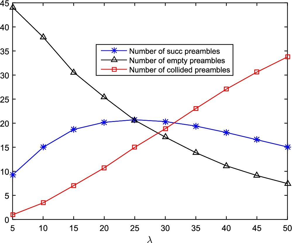
Fig. 1
Average number of preambles chosen by one node, by more than one node and the number of preambles which are not selected by any node.
To find the ACB factor which maximizes the average number of successful transmissions, we equate (
10) to zero. Then, we obtain
In practice, the total number of preambles is 64 in the LTE standard. Therefore, we can approximate
${e^{p/r}}$ with
$1+p/r$. We notice that
p should be between zero and one. Therefore, the optimal ACB factor is obtained as
The information regarding
λ is not available at the eNodeB. Therefore, eNodeB needs to estimate parameter
λ to set the optimal ACB factor. We propose a scheme to estimate this variable. The information which is available to estimate
λ is the number of preambles which are chosen by one node, by more than one node and the number of preambles which are not selected by any node. Figure
1 shows the average number of preambles versus
λ. The results are obtained via simulation of a real system with 25 preambles. The ACB factor is set to 1 for this simulation.
As Fig.
1 shows, for a specific average number of successfully transmitted preambles, there are two values of
λ. Therefore, the number of successful preambles is not a good metric to estimate
λ since it does not provide unique answer. Both the number of empty preambles and the number of collided preambles can be used to estimate the parameter
λ. In this paper, we use the number of preambles not chosen by any node to estimate
λ. The number of collided preambles can also be used for this purpose in a similar manner.
Assume that there are N nodes in a RACH where ACB factor p is used. Let S denote the number of preambles not chosen by node in a RACH. The following theorem characterizes the behaviour of the random variable S in the RACH.
Theorem 1.
The number of preambles which are not chosen by any node follows a Poisson distribution for known N, where N is large.
where $\mu =r{e^{-Np/r}}$.
Proof.
This problem is known as urn problem. Part of our proof is from Feller (
1968), Chapter 4. Let
${A_{m}}$ be the event that
m specific preamble is not chosen by any node for
$m=1,\dots ,r$. Then we have
Let
${S_{m}}$ denote the probability
m preambles are not chosen by any node. This probability can be written as
The probability that at least one preamble is not chosen by any node can be written based on
${S_{m}}$ as
The probability that all the preambles are chosen by the nodes is one minus the probability that at least one preamble is empty. Let
${p_{0}}(N,r)$ denote this probability. Then, we have
Let
${p_{m}}(N,r)$ denote the probability that exactly
m preambles are not chosen by any node. These
m preambles can be chosen in
$\left(\genfrac{}{}{0pt}{}{r}{m}\right)$ ways. The nodes are distributed among other
$r-m$ preambles such that none of the preambles are empty. The number of such cases is
${(r-m)^{N}}{p_{0}}(N,r-m)$. Dividing by
${r^{N}}$, we find the probability that exactly
m preambles remain empty as
The following inequalities show upper and lower bounds for
${S_{v}}$ (Feller (
1968), page 103)
Using the approximation of
${(1-1/x)^{y}}\approx {e^{-y/x}}$, we obtain
For large values of
N and
r, we have
where
$\mu =r{e^{-pN/r}}$. Then, we have
Combining (
18) and (
22), we obtain
This finalizes our proof. □
Let
${s_{1}},\dots ,{s_{k}}$ denote the number of preambles experiencing collision at RACHs 1 to
k. These are considered as
k samples of random variable
S which is proven in Theorem
1 to be a Poisson random variable.
Using the moment generating function of random variable
N, we have
For large values of
r, we approximate
${e^{-1/r}}$ with
$1-1/r$, Then, we have
We also calculate the variance of variable
${s_{i}}$ as
We notice that mean and variance of a Poisson variable are equal. Using the same approximation used for the mean, we have
Let
χ denote the average of random variables
${s_{1}},\dots ,{s_{k}}$ as
The variables
${s_{1}},\dots ,{s_{k}}$ are independent random variables with Poisson distribution. Therefore, we have
To build the estimator, we equate the average of the samples taken from
k RACHs with the mean of random variable
χ which is
${\mu _{\chi }}=r{e^{-\lambda /r}}$. Let
${\tilde{\lambda }_{k}}$ denote the estimation of parameter
λ using information of
k RACHs. Then, we have
Therefore, our estimator would be as
The next theorem shows that the estimator in (
32) is unbiased.
Theorem 2.
The estimator in (
32)
is unbiased. This means, the expected value of the estimation approaches λ as k is large
Proof.
We define function
h as
If we write the second order Taylor approximation of the estimator in (
32) around its mean value, we have
Then, we have
Based on (
36), for large values of
k, the mean of the estimation approaches
λ which proves this estimator is unbiased. □
To show the accuracy of this estimator, we find the variance of the estimation error. The estimation error is defined as
The variance of error can be formulated as
Consider in the first two terms of the Taylor approximation in (
35), we have
We can see that the variance of error approaches zero for large values of
k.
4 Practical Considerations
As the estimator suggests,
k samples are needed to estimate the value of the average traffic rate
λ. Therefore, we need to first choose an ACB factor
p, then estimate the number of tags based on the samples and adjust ACB factor again. An inefficient
p may result in large variance of error. In our proposed algorithm, we first set
$k=1$ and use
$p=1$ to find the estimate of the average traffic as
$\tilde{\lambda }$. Using the obtained
λ, we set the optimal ACB factor as
${p^{\ast }}=\min \{1/(\lambda -1)1\}$. Then, we set
$k=2$ and keep the ACB factor constant for two RACHs. We continue to increase
k and find the optimal ACB factor gradually until we reach the desired
k. We notice that the desired
k is obtained via the desired variance of error. This means, if the desired variance of error in the system should be less than
${\sigma _{\mathrm{threshold}}^{2}}$, then using (
39), the required number of samples
k should be larger than
Another practical aspect that we take into account to modify our algorithm is the drift in the traffic rate
λ. It is possible that during
k RACHs that we use to estimate
λ, the value of
λ changes. If the changes in
λ are considerable, the estimator does not provide useful information. However, if the changes are not significant, one can show that it is possible to modify the estimator in a way that would correct that drift. We assume that the traffic rate drift is Δ between the first RACH and the
$kth$ RACH. We notice that we are interested to estimate the latest traffic rate. We assume that the traffic rate in the first RACH is
$\lambda -\Delta $ while it is
λ in RACH
k. The traffic at RACH
i is
$\lambda -{\delta _{i}}$, where
${\delta _{1}}=\Delta $ and
${\delta _{k}}=0$. We introduce the weighted average of the samples
${s_{i}}$ as
where
${\varpi _{i}}$ is the coefficient of sample
i. We notice that
${\textstyle\sum _{i}}{\varpi _{i}}=k$. In this case, the mean of samples would be
Assuming that all
${\delta _{i}}$s are small, one can approximate
${e^{p{\delta _{i}}/r}}$ with
$1+p{\delta _{i}}/r$. Therefore, we have
This equation shows that to have a correct estimate of
λ,
${\varpi _{i}}$ should be small when
${\delta _{i}}$ is large. Since
${\delta _{i}}$ is large when
i is close to one and then vanishes. The values of
${\varpi _{i}}$ should start from a small number and increase as
i approaches
k. Since
${\delta _{k}}=0$, the highest coefficient is for
$i=k$. Using the first order Taylor series approximation for our estimator in (
32), the mean of the estimated value in this case is
This shows that if we are able to minimize
${\textstyle\sum _{i}}{\varpi _{i}}{\delta _{i}}$, the parameter
λ can be estimated accurately. Algorithm
1 shows the procedure that we use to set the ACB factor.
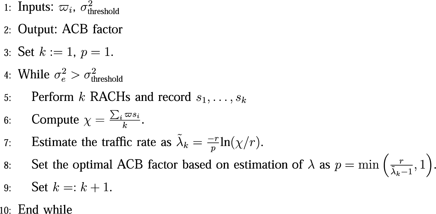
Algorithm 1
Estimation Algorithm
5 Simulation Results
In this section, we present the simulation results and compare the analytical models presented in the paper with the actual results. We validate our models and present the effect and approximations used in the system. The simulation settings for different figures are presented separately.
First, we validate the estimation which is used for the number of successful preambles. Equation (
6) presents the estimation for the average number of successfully transmitted preambles. Figure
2 compares the analytical results and the actual data obtained from simulations. The expected number of preambles transmitted successfully is plotted by changing the value of
λ from 10 to 40. Three different ACB factors are used for simulations, namely 0.5, 0.75, and 1. The analytical results which is an estimation of the actual value are compared with the actual data. We can see that the estimation is accurate in this case.
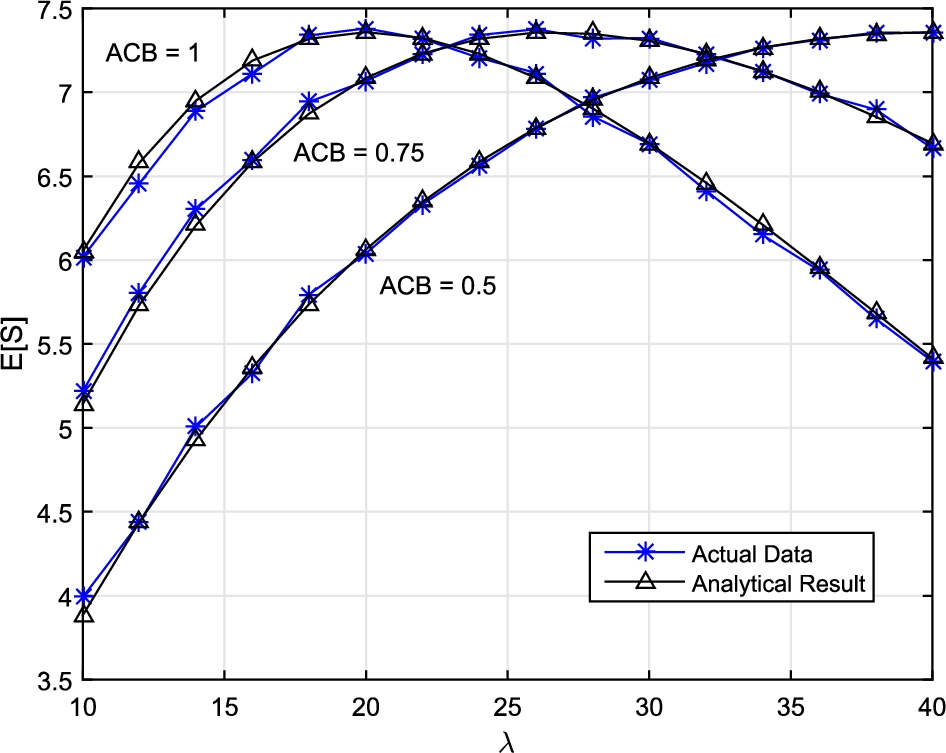
Fig. 2
Average number of preambles chosen by one node.
Next, we investigate the result obtained in Theorem
2. In this theorem, it is shown that the number of preambles not chosen by any node follows a Poisson distribution with mean
$r{e^{-pN/r}}$ when the number of nodes
N is known in the system. In Fig.
3, the mean and variance of this variable is compared with the actual data obtained from simulations. Two different cases are considered for the ACB factor, namely 0.5 and 1. Again, it is shown that the estimation is accurate.
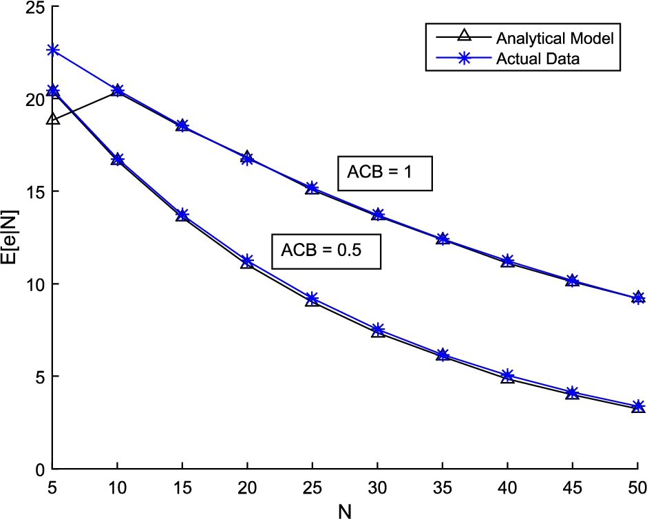
Fig. 3
Actual versus analytical results for the expected number of empty preambles conditioned on N.
Next, we investigate the performance of our estimator. Figure
4 shows the mean of estimated value versus traffic rate. We vary the traffic rate from
λ from 20 to 160. 25 preambles are present in the system. We use our estimator to estimate
λ based on the number of preambles not chosen by any node.
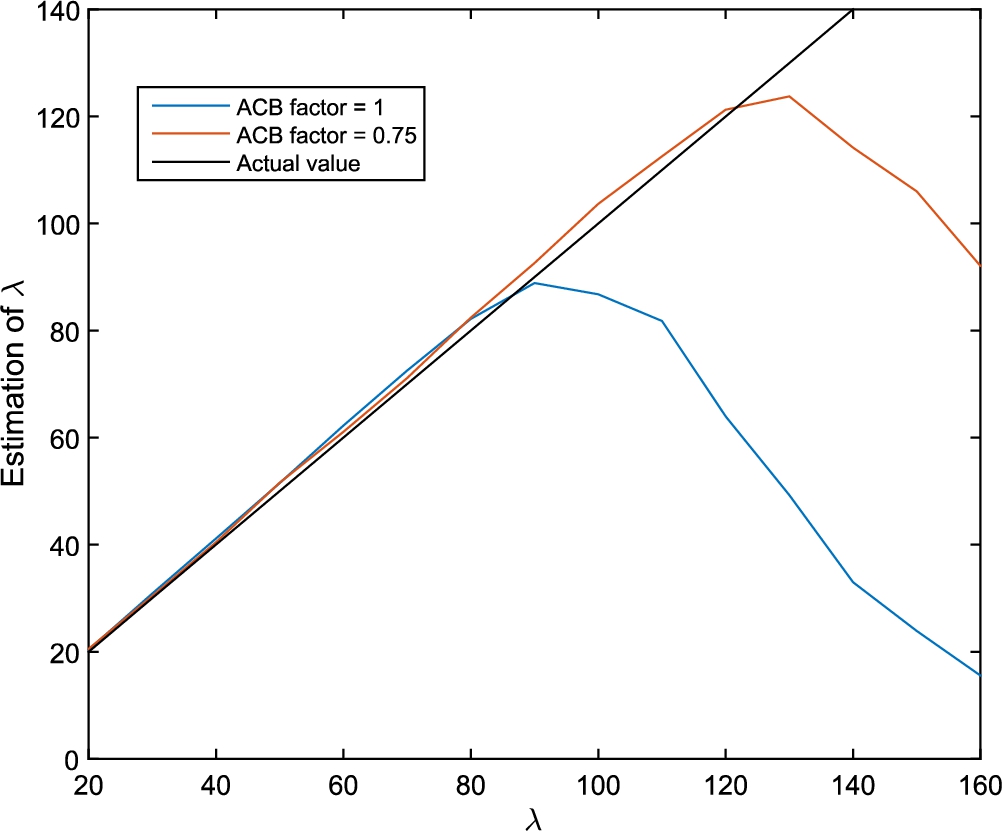
Fig. 4
The estimation of parameter λ.
We use $k=20$ for this simulation. We investigate the effect of k in the next simulations. The simulation contains two curves for two ACB factors, 0.75 and 1. This figure shows the mean of the estimation. When ACB factor is 1, for values of λ below around 80, the estimated value follows the actual value. However, after that the estimated value starts decreasing and shows a bias in the system. The main reason is that as the number of nodes increases, the number of preambles chosen by no node tends to zero. In this case, the estimator fails to estimate and returns no value. In this case, we set the estimated value to 0. This is called the saturation of the estimator. Therefore, the estimator has an operation range which is 80 for ACB = 1 and around 120 for ACB = 0.75 based on the simulation. Within the operation range, the estimator is working well. Outside this range, the estimator is not useful anymore.
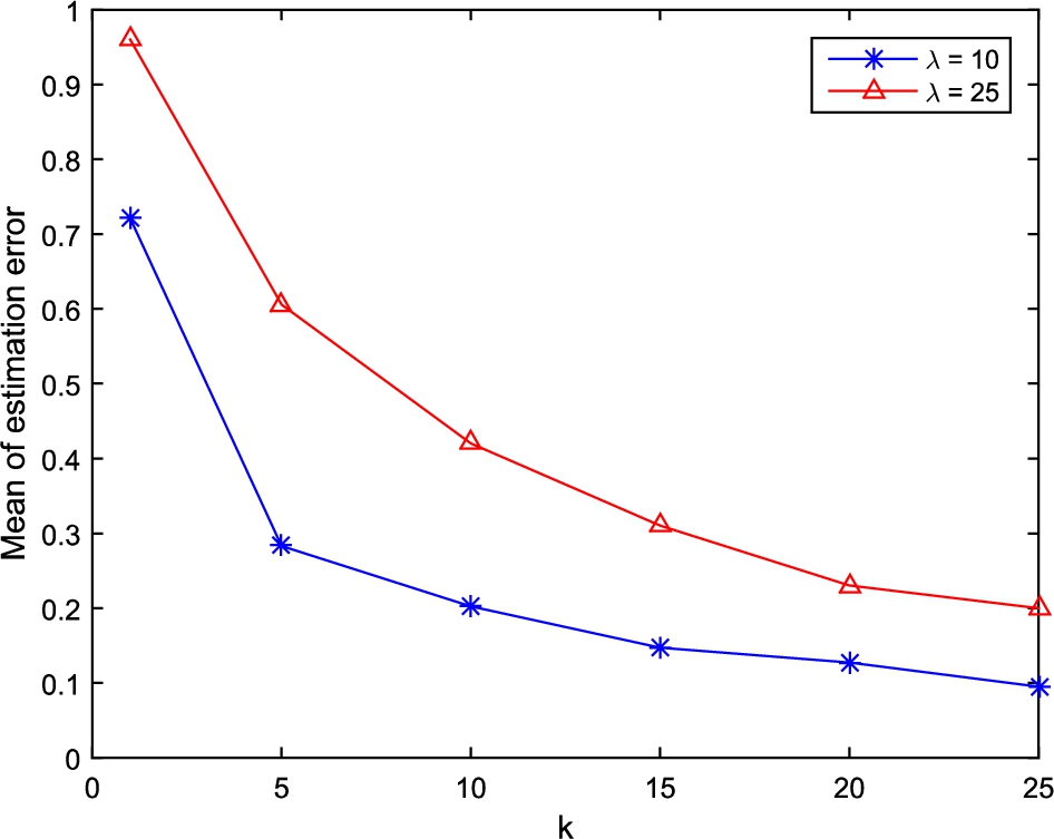
Fig. 5
Mean of estimation error versus the number of samples for two average arrival traffic rates.
We now show that the estimator is unbiased as the number of samples increases. Figures
5 and
6 show the mean and variance of the estimation error as the number of samples increases. The preamble size is fixed to 20 and two ACB factors are set to one. The simulations are carried out for two traffic rates
$\lambda =10$ and
$\lambda =25$. For a fixed number of preambles, we expect that lower traffic rate has better performance in terms of error which can be seen in the figures. Both the mean and variance of error vanishes as the number of samples
k increases in the system. The mean of error falls below 1% and 3% of the actual value when
k approaches 20. If the system can tolerate higher values of error, lower values of
k can be used.
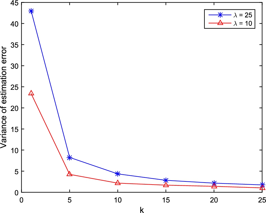
Fig. 6
Variance of estimation error versus the number of samples for two average arrival traffic rates.

