Abstract
As musculoskeletal illnesses continue to increase, practical computerised muscle modelling is crucial. This paper addresses this concern by proposing a mathematical model for a dynamic 3D geometrical surface representation of muscles using a Radial Basis Function (RBF) approximation technique. The objective is to obtain a smoother surface while minimising data use, contrasting it from classical polygonal (e.g. triangular) surface mesh models or volumetric (e.g. tetrahedral) mesh models. The paper uses RBF implicit surface description to describe static surface generation and dynamic surface deformations based on its spatial curvature preservation during the deformation. The novel method is tested on multiple data sets, and the experiments show promising results according to the introduced metrics.
1 Introduction
Computerised muscle modelling garners increasing attention with the rising prevalence of musculoskeletal illnesses (Cieza
et al.,
2020). As of the latest Scopus index, 31 papers on “musculoskeletal illnesses” out of 102 were published after 2020. On the term “musculoskeletal modelling”, there are over one-third of papers published after 2020 compared to the total. This fast development in the field signifies that musculoskeletal modelling approaches play a significant role in musculoskeletal illness treatment. This paper aims to contribute significantly to the field by proposing a new mathematical muscle description. To provide context, we begin with a brief overview of the evolution of critical contributions.
Muscle modelling has a rich history, with Hill (
1938) presenting the first formal mathematical representation, a three-element model for muscle fibre. As technology advanced, the need for precision led to the development of more intricate models. Initially, fibres were individually represented, as seen, e.g. in the alpine skiing context (Heinrich
et al.,
2023). Subsequently, a “Via-points approach” emerged, linking multiple fibres in series, e.g. in shoulder muscle modelling (Abderrazak and Benabid,
2022).
While these methods often operate in one dimension, moving to higher dimensions, especially in 2D space, evolved crucial because the 1D model cannot accurately define the original shape, producing errors up to 75% (Valente
et al.,
2012). Employing 2D space allows the description of muscles using surfaces, a more intuitive technique for reflecting external structures. This paper focuses mainly on 2D models, as detailed in Section
2.
The open, ultimate problem is developing an accurate, simple, fast, and smooth musculoskeletal model using the least possible parameters. All of the state-of-the-art methods lack one or the other or give some compromises.
The paper primarily emphasises a detailed description of two-dimensional techniques, allowing faster calculations while keeping the ability to infer internal muscle composition. Two main objectives include achieving more immediate model deformation with fewer updated parameters and data reduction. The goal is achieved using a mathematically described RBF implicit surface geometric model, providing infinitely differentiable smooth surfaces and using fewer parameters than the “traditional” triangular mesh approaches.
The contribution of this paper lies not just in the overall RBF model but also in a novel metric to determine the approximation accuracy presented. This metric can also be used in different research fields where two surfaces must be compared. The RBF solver is another contribution, and its usage can also be extended to applications where some smooth objects (without sharp edges) need to be approximated, such as fluid dynamics, aerodynamics, computer graphics and more.
Section
2 describes various models already used for muscle modelling, followed by Section
3, including the description of RBF in general and muscle modelling. Section
4 then describes the paper’s contribution to static and dynamic models. Finally, in Section
5, experiments prove the model works as expected in theory.
2 Related Methods
Having established the theoretical background, we now advance to a detailed investigation of some techniques relative to muscle modelling.
The origin of a musculoskeletal model is deeply rooted in empirical data. The primary raw materials for these models are medical scans, such as Magnetic Resonance Imaging and Computed Tomography screenings, originating from living subjects and cadavers. Recently, the processing has evolved, transitioning from semi-automatic to fully automatic techniques. This progression involves the segmentation of images, a critical step where the relevant structures, such as bones, joints and muscles, are isolated and extracted from the rest of the image.
2.1 Bones and Joints
Following segmentation, surface models of bones are created. This process is not just about assembling a skeletal structure; it involves the intricate specification of joints, setting constraints on the degrees of freedom within these joints. Here, e.g. the STAPLE algorithm by Modenese and Renault (
2021) can significantly automate and streamline the process.
Triangular meshes are the most common way to approximate bone surfaces by connecting triangles to define the object’s overall shape. The methodology for obtaining a triangular muscle model from a person entails a comprehensive process that begins with acquiring high-resolution, segmented medical images, commonly from MRI or CT scans. These images provide a detailed view of the bones (and surrounding tissues). The next step involves the extraction of a triangular mesh from these segmented images, a task typically accomplished using algorithms such as Marching Cubes (Lorensen and Cline,
1987) or Marching Triangles (Hilton
et al.,
1996). These algorithms traverse the voxel grid of the images, forming vertices, edges, and faces that approximate the bone surface, effectively converting the 2D segmented images into a 3D surface representation.
Following the initial mesh extraction, the mesh undergoes a series of refinement procedures to enhance its quality and anatomical accuracy. These procedures include the removal of non-manifold vertices and edges to eliminate anomalies that do not adhere to the criteria of a well-defined surface. Concurrently, any gaps or holes in the mesh are meticulously filled to ensure continuity of the bone surface, a critical step for maintaining anatomical fidelity. The mesh is further refined by optimising the shapes of the triangles to more accurately align with the bone’s contours and by reducing the mesh to lower its complexity while keeping the model’s overall shape and intricate details.
Additionally, Laplacian smoothing is applied to the mesh. This process adjusts the position of each vertex based on the average of its neighbouring vertices, effectively smoothing out irregularities and noise, resulting in a uniform and more realistic representation of the bone. The refined mesh is then rigorously reviewed and compared against the original segmented images by medical professionals to validate its accuracy, ensuring the model precisely mirrors the anatomical structure.
While the forces used on bones during the movement can induce deformations, these deformations are generally so minute that, for practical purposes, they can be disregarded. This assumption yields the bones as rigid bodies in motion. This assumption is in contrast to the muscle-tendon units.
2.2 Muscles and Tendons
Joint data about the muscles and tendons (together form muscle-tendon units – MTU) is acquired because it is difficult to distinguish the muscle and the tendon apart from the imaging; otherwise, the data can be obtained in the same fashion as in the case of bones. However, the problem is that these tissues are less visible in the imaging. Fortunately, the segmentation can also be automated, but more complex strategies are required, with machine learning methods emerging as promising approaches (Goyanes
et al.,
2024). Despite their potential, these techniques have yet to become a staple in routine practice, and semi-automatic approaches are used instead.
If the deformation is discussed, muscles behave differently than bone structures; they exhibit elastic deformations, presenting a significant challenge in modelling their behaviour accurately to the known movement of bones. Various models attempt to address this, often employing many oversimplifications.
Also, in the real-world scenario, muscle deformation results from the contraction or relaxation of muscle fibres, driven by the sliding of actin and myosin filaments within muscle fibres. This contraction leads to changes in muscle shape, causing deformation. In inverse kinematics, muscle deformation is pretended to be caused by adjacent bone movement, posing the challenge of figuring out the shape of unknown parts of the muscle model. If we do not consider measurements of the physiological signals (e.g. electromyography), it is required to perform the inverse kinematics because the bone displacements are known; however, the shape of the muscles during the movement is not (due to the problematic data acquisition).
The first models created were one-dimensional and were formed by a straight line, polyline, or curve and their multiples.
2.2.1 1D Models
The simplest models might represent a muscle as a straight line connecting two points on different bones, blatantly ignoring any potential intersection with the bone itself. This approach relies heavily on the assumption that the attachment points are accurately chosen (Kohout and Cervenka,
2022). A slight improvement to this model is to replace the straight line with a polyline or a curve that either passes through predetermined points relative to a bone or traces the surface of a parametric body, aiming to minimise the curve length. However, fine-tuning these models to mirror reality is arduous (Hájková and Kohout,
2014).
It’s also imperative to represent muscles not just as mere lines or curves but as substantial higher-dimensional models (Kedadria
et al.,
2023) to enhance the realism of musculoskeletal models.
2.2.2 3D Models
Geometrical 3D models have been explored, utilising the fact that a large set of muscle fibres creates the muscle. Modelling approaches using mass-spring systems (Janák and Kohout,
2014) and the finite element (FE) method are currently gaining prominence (Delp and Blemker,
2005). The FE method, utilising a template of internal structure projected onto the surface shape, proves superior accuracy. The main issue of those methods is their large number of parameters, which need to be figured out, and their computational complexity. Therefore, this paper concentrates more on the two-dimensional (surface) models instead, which is a reasonable compromise between a simple but inaccurate 1D modelling and 3D accurate but too complex 3D modelling (Macklin
et al.,
2016).
2.2.3 Discrete 2D Models
Despite muscles lying in the 3D space, modelling them in lower dimensions is viable. Straight lines or polylines can be employed in one dimension but inaccurately. In two dimensions, already obtained triangular surfaces are limited in the original object description but can be accurate enough. Each “well-behaved” 3D surface model constructed by a single component manifold can be parameterised in two dimensions or described utilising a 2D representation.
In the case of model dynamics, numerous approaches have been developed, primarily working directly on the triangular meshes that have already been obtained. Here, we provide a brief overview of the most significant ones.
Position-Based Dynamics. Position-based dynamics, introduced by Müller
et al. (
2007), is a rapid technique widely utilised in the animation industry for simulating deformations of elastic objects. Initially created for generic shapes, the method inputs a smooth manifold surface mesh and generates its deformed counterpart.
An extended version, XPBD (Macklin
et al.,
2016), introduces the concept of elastic potential energy, removing the need to determine time steps and iteration counts. XPBD has been applied to muscle modelling challenges by Romeo
et al. (
2018), who addressed limitations regarding convergence speed, setup simplicity, intuitive controls, and artistic control. They constructed an internal structure inside the surface mesh, accounting for muscle anisotropy. However, the approach lacked attention to collision detection and resolution, later addressed by Cervenka
et al. (
2023).
In 2019, Angles
et al. (
2019) introduced an XPBD-based method for muscle modelling, virtually decomposing the muscle into flexible “rods” approximating muscle fibres. These rods adjust their diameter to maintain volume, enabling real-time simulation. The main issue is the same: the problem of muscle-bone penetration is not adequately addressed or apparent in the paper or its supplementary material.
As-Rigid-as-Possible Surface Modelling. The as-rigid-as-possible approach (ARAP), developed by Sorkine and Alexa (
2007), is a technique for determining minimal non-rigid transformations in a surface mesh. Unlike the method by Kellnhofer and Kohout (
2012), which involves volume constraints and an internal skeleton, “it distinguishes itself by not requiring an internal structure”. Fasser
et al. (
2021) applied ARAP in a medical context to morph the template of a pelvic bone onto subject-specific landmarks, though overlooking certain critical features like volume preservation. Wang
et al. (
2021) investigated ARAP but chose not to use it due to non-smooth shapes and spikes in results. ARAP has also found application in time-varying meshes by Dvořák
et al. (
2021).
ARAP minimises shape deformation by discouraging non-rigid transformation via a cost function. Mathematically, this is characterised as the search for a solution to a nonhomogeneous system of linear equations. The matrix corresponds to the discrete Laplace operator of the mesh, while the right-hand side vector encompasses the second differences of each vertex concerning its neighbours.
The main drawback of ARAP and similar approaches lies in recalculating each mesh parameter in every iteration, proving time-consuming for fine triangular meshes. Also, the triangular mesh has the smoothness issue mentioned before. Therefore, a continuous 2D model better approximates smoothness and is better suited for the deformation approaches.
2.2.4 Continuous 2D Models
The Non-Uniform Rational Basis Spline (NURBS) is an interpolation and approximation method (Nie
et al.,
2022) describing a surface via a set of B-spline curves. NURBS is useful for interactive applications, offering higher smoothness than triangular meshes, allowing intuitive deformation of specific parts of the geometrical model (see, e.g. Clapés
et al.,
2008 or Sánchez-Reyes and Chacón,
2020). For muscle modelling, the NURBS is not required to form a structure as triangular meshes when creating the data and then approximate those data, meaning that after applying the Marching Cubes or Triangles step, the vertices will not be connected by triangles but rather by individual NURBS patches and the smoothness is accomplished automatically. Also, if a part of the segmentation is missing, the NURBS techniques can restore those parts more precisely than in the triangular mesh case.
D-NURBS (Terzopoulos and Qin,
1994) (Dynamic-NURBS) can be used for dynamics. It extends the NURBS approach by incorporating physical phenomena for more intuitive interactive shape deformation relevant to various purposes such as high-resolution digital terrain (Ye
et al.,
2020), virtual reality (Lavoie
et al.,
2006), or CAD applications (Zhang and Qin,
2001).
Ni
et al. (
2023) used D-NURBS for muscle shape parametrisation and deformation. They achieved satisfactory results by defining muscle shape with a set of neighbouring 2D NURBS plates, reaching a mean square difference of approximately 1.5 mm and a maximum volume error of 0.75%.
While these approaches offer valuable insights, a common challenge is recalculating every parameter in each iteration, which can be time-consuming. Also, the neighbourhood of vertices needs to be defined for all the techniques mentioned.
3 Radial Basis Functions
Even the previously described NURBS techniques require some relations between the vertices (neighbourhood), but Radial Basis Function (RBF) techniques do not require that knowledge. The task of estimating and fitting scattered data is widespread across various fields of engineering and scientific research. To list only a limited subset of the RBF usage possibilities, Zhang
et al. (
2022) shows its usability for better predicting the subcellular location of long non-coding RNA. Oliver and Webster (
1990) demonstrates this by applying the kriging method for interpolating geographical data, while Kaymaz (
2005) demonstrate its effectiveness in solving issues related to structural reliability. The process has further applications in simulation, e.g. in Sakata
et al. (
2004)’s study on wing structures or Joseph
et al. (
2008)’s development of metamodels. RBF techniques address partial differential equations, especially in engineering.
The RBF method was presented by Hardy (
1971) and improved by him (Hardy,
1990) later. Majdisova and Skala (
2017) have offered different strategies for RBF positioning. Significant studies have been conducted in terms of ‘shape parameters’ in RBF approaches, including, e.g. search for optimal settings by Wang
et al. (
2021), investigations by Afiatdoust and Esmaeilbeigi (
2015), and research into varying local shape parameters methods by Cohen
et al., Sarra
et al., and Skala
et al. (
2020).
The radial basis function approach uses “centre points” instead of surface vertices, serving as descriptors for spatial function locations. Unlike NURBS, modifying a single RBF centre location can affect the entire surface because of its “blending” behaviour with other RBFs nearby, propagating recursively throughout the volume. To address the RBF placement possibilities, Majdisova and Skala (
2017) conducted a comparative study of various RBF placement strategies, showing that uniformly sampled input functions tend to lead to ill-conditioned RBF equation systems. They seek the solution by proposing a quasi-random sampling, such as the Halton distribution. Alternative methods have also been suggested, such as regularisation by Orr (
1995) and enhancements close to function boundaries by Wright (
2003).
The RBF approach offers advantages over triangular mesh representations of muscle surfaces, including:
-
• There is no need to define the connectivity between control points.
-
• RBFs can generate ${C^{n}}$-smooth surfaces, with the user-defined required degree of smoothness denoted by n.
-
• RBF may use fewer parameters compared to triangular meshes in general.
-
• Deforming a muscle may involve changing only a portion of the parametric space while maintaining smoothness.
For each application, the correct RBF must be chosen first to reach desirable properties and satisfactory results. Two global RBFs are commonly considered: the Gaussian RBF or thin-plate spline (TPS). The Gaussian RBF is defined as
${e^{-\alpha r}}$, and TPS as
${r^{2}}\log r=\frac{1}{2}{r^{2}}\log {r^{2}}$. The decision of which one to use cannot be made by the differentiability criterion (because both are infinitely differentiable). The Gaussian can also be adjusted using the shape parameter; however, TPS (in its original form) cannot. There are also other options for global RBFs (such as in Skala and Cervenka,
2019) to consider; however, Gaussian RBF and TPS provide stability and a good understanding of their behaviour and are already the most analysed by others.
3.1 Mathematical Description
A single RBF is a mathematical function defined solely by the distance from a designated point, denoted as the centre. Mathematically, it can be expressed as $\varphi (\| {\mathbf{x}_{i}}-{\boldsymbol{\xi }_{j}}\| )$, where ${\boldsymbol{\xi }_{j}}$ represents the centre point’s coordinates, and ${\mathbf{x}_{i}}$ is an arbitrary independent point.
The expression of RBF approximation, defining the function value at any specific input points, is as follows:
Here, the approximation
h at the location of
${\mathbf{x}_{i}}$ is described by
${r_{ij}}=\| {\mathbf{x}_{i}}-{\boldsymbol{\xi }_{j}}\| $ the distance between the input point
${\mathbf{x}_{i}}$ and the centre point
${\boldsymbol{\xi }_{j}}$; and
${\boldsymbol{\lambda }_{j}}$ is the weight of a single RBF
φ, which can be, e.g. already discussed Gaussian RBF or TPS. The equation (
1) can be formulated in a matrix form, resulting in a square matrix
A within the system of linear equations. A simple example of RBF approximating a function can be seen in Zhao and San (
2011).
The idea can be extended using polynomial conditions, which can improve accuracy. The extended system of equations, considering these conditions, is expressed as:
Here,
P are the polynomial conditions,
$\boldsymbol{\lambda }$ represents RBF weights, Big
A is the RBF matrix without the polynomial constraints, small
a contains resulting coefficients of the polynomial, and
h encompasses values at the input points.
Suppose we disregard the polynomial conditions for a while. In that case, RBF approximation involves solving the equation (
1). The equation can also be described as an overdetermined system of linear equations
$\mathbf{A}\mathbf{x}=\mathbf{b}$, where
A is a rectangular matrix,
b and
x are vectors, and the number of rows
N is greater than the number of columns
M.
The Ordinary Least Squares (OLS) method can choose weights
${\lambda _{j}}$, minimising mean square error (MSE). This involves computing weights utilising the inverse or pseudoinverse:
$\boldsymbol{\lambda }={({\mathbf{A}^{T}}\mathbf{A})^{-1}}{\mathbf{A}^{T}}\mathbf{h}$. Although typically satisfactory, OLS can encounter stability problems, as noted by Skala (
2017), which needs to be kept in mind while solving. It is often beneficial to even choose another solver instead. Furthermore, an issue when combining values of different units in the OLS method to solve the equation system with polynomial conditions emerges, which needs to be properly addressed (Skala,
2017). The different units can be found in matrices
A and
P, see equation (
2).
3.2 RBF for Muscle Modelling
Due to the often intricate shape of muscles/bones (e.g. with many triangles, quadrilaterals, etc.), approximating the muscle/bone rather than interpolating, is advantageous for subsequent calculations. When approximating, spatial placement of individual RBF is critical. A naive approach involves uniformly sampling the input shape (scalar distance field of the volumetric data or triangular mesh in the case of muscle modelling), but this may not adequately capture the muscle/bone underlying properties.
Even though utilising the polynomial conditions improves the outcomes and enhances the matrix conditionality in some cases, the presumption is that the input data behaves like the selected polynomial. However, this is not the case in muscle modelling, where the data’s overall shape resembles somewhat an ellipsoidal shape rather than a polynomial form, further diminishes the relevance of polynomial constraints, which will not be discussed further.
4 Novel RBF Mathematical Model
The number of parameters of the triangular mesh is often large. To address the issue of reducing parameters during deformation, a new mathematical model is proposed, encompassing both static muscle shape and its dynamic configuration during bone movement.
4.1 Geometrical Static Model
Even though the number of parameters will be reduced, many will still be present. Therefore, the extensive emerging RBF linear equation system would be ill-conditioned. The static model is constructed using a greedy approach, adding one RBF after another to solve the issue. In each iteration, the algorithm identifies the position and shape of a single RBF to minimise the approximation error effectively.
The objective is to minimise the squared error of the approximation to the original triangle mesh across all vertices throughout the bounded space
$\Omega \subseteq {\mathbb{R}^{d}}$:
Here, N denotes the current number of employed RBFs, k is the number of vertices in the triangular meshes, d is the number of dimensions, and ${\mathbf{v}_{j}}$ is the respective vertex. The notation $\| \mathbf{x}{\| _{2}}$ represents the L2 norm of a vector x.
Creating the geometrical static model initiates the generation of a scalar distance field (SDF) on the triangular mesh. This field is later sampled using a (quasi-)random sampling method. Throughout the research, various distributions, including uniform, random uniform, Gaussian, and Halton, were tested. The findings indicated that the Halton distribution emerged as the most effective option, which is following other research (see, e.g. Majdisova and Skala,
2017; Cervenka
et al.,
2019). The overall result of the model generation can be seen in Fig.
1.
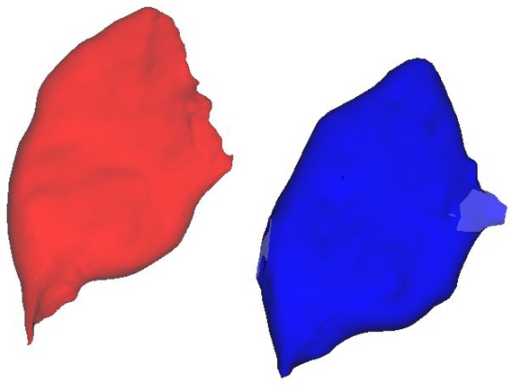
Fig. 1
The geometrical static model depicts a gluteus maximus muscle. The red represents the original triangular mesh, while the blue represents its RBF approximation.
4.1.1 RBF Placement
In this study, we followed the placement of each RBF by Carr
et al. (
2001), placing centres at the three level-sets of the isosurface. However, in the case of muscle modelling, only a subset of the proposed set is required. This subset is determined through a straightforward trial-and-error method. It involves evaluating an objective function and dynamically minimising it. Therefore, this placement approach can be described as greedy. The process involves checking the objective function of each RBF for every vertex across all samples within the input space (the bounding box of a mesh), as well as for each predefined shape parameter (refer to Section
4.1.2 for more details).
Greedy placement is a sub-optimal approach because two independently and subsequently placed centres independently select a shape parameter for each RBF compared to two “cooperating” centres, which are not required to be optimal at the time of their selection. However, this approach avoids the stability issue by using an extensive system of linear equations as a solution.
The optimal position is for each centre selected, and the RBF function is subtracted from the volume bounded by, e.g. the AABB box and the process is iterated until either the allotted number of RBFs is utilised or the predetermined level of accuracy is achieved. This centre point distribution approach was designed to avoid the OLS stability issue altogether.
4.1.2 Shape Parameter Selection
Choosing the radius of action, also called a shape parameter, is pivotal in achieving precise interpolation or approximation. While one option is to independently select a shape parameter for each RBF, this can lead to many stored parameters. On the other hand, determining an optimal global shape parameter for all RBFs leads to inaccuracies and using it as a compromise remains an open question. Different approaches have been suggested, such as those by Wang
et al. (
2021), Afiatdoust and Esmaeilbeigi (
2015), and Sarra and Sturgill (
2009). Still, they may not always identify the optimal shape parameter for each RBF. During testing, we discovered that the single global shape parameter is not exhaustive. Search from a limited list of possible shape parameters is suitable because the number of parameters is low. The condensed set of parameters reduces the storage capacity and computational complexity while searching for the most suitable one.
4.1.3 Objective Functions
The task at hand for evaluating the placement of individual RBFs is to assess how accurately the placement represents the original shape. One possible metric for this assessment is the Jaccard index; the second is the mean square error.
Jaccard Index. The Jaccard index quantifies the disparity in volume between two objects: the original mesh and the surface formed by RBF. It is mathematically defined as follows:
In this context, i represents the intersection volume, u symbolises the union of both meshes and d represents the difference between both meshes. Calculating the exact volume of intersections can be complex so that a rough approximation might be a more practical choice. Rather than using volumes, the number of samples (using the already described Halton distribution) in each group can be used. A higher number of samples leads to more significant computational accuracy. It is worth noting that while the Jaccard index helps specify the difference between two shapes, it does not provide an understanding of how much is “inside” or “outside” something, which is a feature to consider.
Mean Square Error. The Mean Square Error (MSE) provides a more detailed insight into both muscles’ interior and exterior rather than a binary assessment. Calculating MSE requires knowledge of interior information. Interestingly, no additional information is necessary for the RBF representation, as it can be evaluated at any point within the volume. For the original surface mesh, interior information can be acquired using a scalar distance field (SDF) already obtained for its creation, allowing us to determine the distance of each vertex from the surface mesh.
The computation of the MSE objective function entails integrating the squared L2 norm across the subset Ω of the original space
${\mathbb{R}_{d}}$ and can be expressed as:
Here, the function s represents the Scalar Distance Field (SDF) constructed over the mesh, while h represents the sum of all currently utilised RBFs. When computed, a more efficient approach is subtracting each RBF from the function s and then calculating the updated s norm.
It’s important to note that these objective functions may encounter challenges when dealing with the translational motion of the shape. This paper assumes that the muscle movement occurs only in part of the muscle while the rest remains static (for instance, the muscle is attached to two bones, but only one moves). This assumption holds as long as the deformation of a muscle is done in the local scope, with one static and one moving bone (meaning both bones cannot translate together during deformation).
Delving further into the challenge of selecting the appropriate objective function, opting for the MSE tends to yield a smoother surface. At the same time, the Jaccard index aligns more closely with the original model at the expense of introducing a less smooth surface. Hence, a combination of both proves to be a favourable approach.
4.2 Metrics
The metric used to compare the original surface with a new one is a weighted sum between the Jaccard index and MSE. This metric is proposed because the smooth surface provided by MSE and the surface location accuracy provided by the Jaccard index are required. The weight
σ is called a
smoothness factor:
The equation calculates the final metric ${C_{m}}$ using the smoothness factor σ, Jaccard index ${J_{i}}$, and MSE value denoted as ${M_{se}}$. The Jaccard index is expressed as $1-{J_{i}}$ to penalise the lower Jaccard index more than the higher one. The MSE variable ${M_{se}}$ must also be normalised into zero to one interval, which is accomplished by dividing the MSE total value by the maximum one possible.
4.2.1 Regularisation
Regularisation optimises how the RBFs are placed, increasing the likelihood of placing RBF centres in a predefined position or formation. When forming the RBF surface, it may be advantageous to position RBFs within the muscle volume and less outside, resulting in a more accurate curvature field, including fewer local extrema near the surface. The central concept involves penalising the RBFs placed significantly outside the desired region more heavily than the others.
When utilising the Signed Distance Field (SDF), the sign indicates whether the target vertex is inside or outside. Let’s denote the signed distance as ${d_{{\mathbf{v}_{i}}}}$. To obtain relative values rather than absolute distances, we can divide ${d_{v}}$ by the maximum possible distance ${d_{\text{max}}}$. This yields ${r_{d}}=\frac{{d_{{\mathbf{v}_{i}}}}}{{d_{\text{max}}}}$, which falls within the interval $(-\infty ,1)$.
Additionally, to enable the use of wider RBFs (avoiding the potential replacement by less advantageous numerous RBFs with minimal overall influence), a similar penalisation for the RBF shape parameters can be implemented: ${r_{s}}=\frac{{\alpha _{i}}}{{\alpha _{\text{max}}}}$. Since $\forall i,{\alpha _{i}}\gt 0$, the ${r_{s}}$ value will fall within the interval of $(0,1)$. The wider RBFs are then useful in forcing fewer parameters to move to deform the overall shape.
To summarise, the parameters for the following need to be determined. The regularisation factor
γ represents the ratio of how much of the original cost function is employed.
4.3 Mathematical Dynamic Model
In our studied scenario, the bones undergo a rigid transformation in inverse kinematics, typically following the desired real-world movement. Subsequently, in an inverse manner, the shape of all the muscles related to the bone needs to be reconstructed. The portions of the muscle attached to the bones are mandated to move in conjunction with these bones, while the remaining parts of all muscles require reconstruction. In the following text, the muscle is meant to be the whole muscle-tendon unit to ensure that the “muscle” is correctly attached to a set of bones. Also, for the simplicity of the following text, just a singular muscle involved in deformation is considered.
The main idea of the novel dynamic model is to find a new shape according to the curvature of the original one, preserving its initial shape as much as possible. The mathematical description to maintain the initial shape as much as possible can be described in many ways. In the case of muscle modelling, the muscle’s initial curvature throughout the whole volume is a suitable shape descriptor. Mathematically speaking, we define the cost function as the total difference of the original (
${\kappa _{\mu {f_{\text{i}}}}}$) and current curvature (
${\kappa _{\mu f}}$) over the bounded space
$\Omega \subseteq {\mathbb{R}^{d}}$, and we are looking to obtain its gradient:
Then we use the definition of the 3D RBF approximation (and for the sake of simplicity, use
${g_{i}}$ as the individual weighted RBF):
To calculate the curvature, we need to find the eigenvalues of the Hessian matrix of f, also the calculation of second partial derivatives of f is needed. From the Hessian matrix, all of the eigenvalues can be obtained.
For this paper, only global RBFs were considered at first due to their influence over the entire space, allowing the change of the whole model by altering fewer parameters. Moreover, for that purpose, the global Gaussian RBF is chosen for this paper due to its simplicity if differentiation is considered, which is beneficial when creating this dynamical model. If the Gaussian RBF is considered, then the mean of all of the eigenvalues can be calculated as:
Combining (
10) and the gradient of (
8), the complete cost function can be expressed as:
The calculation, including all the computational steps, can be found in Appendix
C. The result implies that the direction of the gradient depends on the following factors:
-
1. $({\kappa _{\mu f}}-{\kappa _{\mu {f_{\text{i}}}}})$ – the direction of the gradient is influenced by the disparity between the original and new curvature across the entire interval. The more significant this difference, the larger the magnitude of the gradient.
-
2. ${\alpha _{i}^{2}}$ – the shape parameter plays a crucial role. A broader function exerts a more significant influence on the gradient of the respective centre point ${\xi _{kj}}$.
-
3. ${g_{i}}(\mathbf{x})$ – naturally, the RBF itself plays a significant role.
-
4. $({x_{j}}-{\xi _{kj}})$ – as we integrate further from the centre point, its impact diminishes.
-
5. $(2{\alpha _{i}}\| \mathbf{x}-{\boldsymbol{\xi }_{i}}{\| _{2}^{2}}-2-d)$ – the distance of the current RBF to the integration variable is not just significant exponentially in ${g_{i}}$ (expressed in third point) but also linearly (subject to specific constant manipulations).
The new mathematical model for the RBF shape deformation defines where all centre points should be translated (in the direction specified by its gradient). At this point, we can, according to the broader shape parameters and larger weights, decide which RBFs are more significant and calculate the deformation more often. In contrast, the less critical parameters can be recalculated only a few times, which may reduce the computational complexity significantly.
It’s crucial to re-emphasise the centrality of our mathematical model in this study. Even though this paper does not adequately address any collision detection and response (CD/R) issues, similar techniques to Cani-Gascuel and Desbrun (
1997) hierarchical CD/R can be used in the future. This section has encapsulated the theoretical and practical applications of radial basis functions in muscle modelling and illuminated the robustness and versatility of our mathematical approach. Through rigid exploration of complex mathematical concepts and their biomechanical applications, this research emphasises the potential for advanced modelling techniques in future studies, paving the way for groundbreaking innovations in biomechanics and beyond.
5 Experiments
The proposed approach has been tested to ensure its usefulness for musculoskeletal modelling. Here, we detail the critical experiments conducted to test the relevance and efficacy of the radial basis function approach in muscle modelling, concentrating on processes and their implications for our theoretical description.
The mathematical model of the curvatures can be evaluated using actual data from the gluteus maximus, gluteus medius, iliacus and adductor brevis muscles. The initial experiment will be conducted without regularisation, solely relying on the greedy placement approach.
5.1 Geometrical Static Model
Before we dive deeper into the muscle dynamics experiments, the first experiment shows the results of the static model. These experiments prove the correct centre placements.
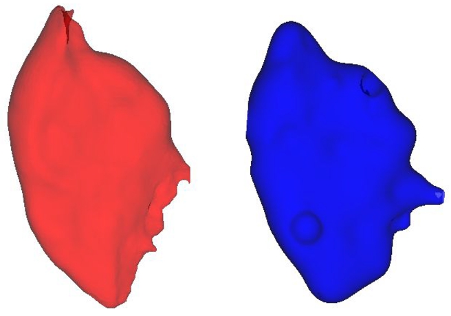
Fig. 2
The original gluteus maximus muscle in red and its RBF counterpart in blue.
5.1.1 Greedy Centre Placement
Using a greedy approach, we employ a naive RBF placement strategy in the initial experiment. The results of such placement can be seen in Figs.
2,
3,
4 and
5. While this approach is straightforward to implement and relatively fast in execution, as depicted in Fig.
11, it exhibits issues with numerous small (but still different in size) RBFs distributed across the entire space. The approach forms a complex curvature field with numerous potential local extrema. Additionally, the curvature outside the muscle boundaries (though barely visible in the image) is cluttered with unneeded curvature differences, further exacerbating the proliferation of local extrema. The problem is solved with regularisation, and the next section describes the experiment.
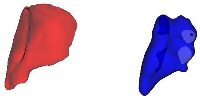
Fig. 3
The original gluteus medius muscle in red and its RBF counterpart in blue.
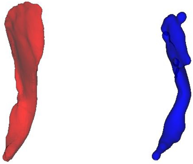
Fig. 4
The original iliacus muscle in red and its RBF counterpart in blue.
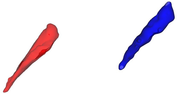
Fig. 5
The original adductor brevis muscle in red and its RBF counterpart in blue.
5.1.2 Regularisation
By including the regularisation term, higher curvatures will be concentrated at the borders of the original triangular mesh. The regularisation creates more promising conditions for the gradient descent method to achieve a superior approximation of the muscle in motion, mitigating the problem of numerous local minima in the field. Three examples are presented here: one with a regularisation factor of 0.7, another with a factor of 0.3, and the last with a regularisation factor of 0.05. The outcomes can be observed in the Appendix
A in Figs.
12,
13, and
14, respectively.
5.1.3 Metrics
The weighted metrics (between the MSE and JI) have been tested with two weights (0.15 and 0.85) and on two different sample resolutions (10k and 100k vertices). The evaluation for the first hundred RBF centres is shown in Fig.
6, which describes the initial part of the metrics convergence.
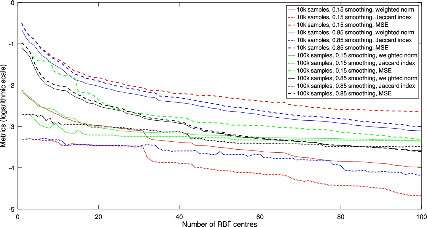
Fig. 6
The metrics evaluation on gluteus maximus muscle up to 100 RBF centres, with different sampling density and smoothness weight.

Fig. 7
The metrics evaluation on gluteus maximus muscle, with different sampling density and smoothness weight.
One may tell from the results that both metrics converge similarly, and in the end, they tend to go to a fixed value. However, if you continue further, it will be evident that this is not the case because the penalisation of the Jaccard index holds near a fixed value. Still, after a while, it goes faster towards zero (on a non-logarithmic scale). The results for more (7000) centres are visualised in Fig.
7. The other takeaway is that the finer the sampling (green and black dotted curves), the longer it takes to lower the penalisation of the Jaccard index (red and blue). Also, the lower the smoothing factor (red and green), the higher the MSE (dashed lines), confirming that both metrics describe the shape difference significantly differently.
5.1.4 Limitation
A well-known problem with the static surface RBF approximation is its ineffectiveness in accurately approximating sharp edges. This drawback is less critical in muscle modelling, as most soft tissues are relatively smooth and do not possess sharp edges, often resembling spherical shapes. However, this issue can be demonstrated using a simple 3D volumetric shape like a tetrahedron. A tetrahedron has six sharp edges (each with a dihedral angle exceeding 70 degrees) and four corners, which present significant challenges for RBF approximation.
The fundamental issue with RBFs is that each RBF inherently forms a spherical isosurface at a given value. To create a sharp corner would theoretically require an infinite number of infinitesimal RBFs. An example of attempting to develop an RBF static surface for a tetrahedron is shown in Fig.
8. Let’s also note that in the case of the tetrahedron and similar shapes, often no data reduction is achieved, but rather the opposite.
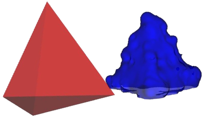
Fig. 8
An attempt to create an RBF surface for a tetrahedron demonstrates the unsuitability of RBF for approximating sharp edges. RBF is ineffective for shapes like a tetrahedron due to its inability to model the sharp edges accurately.
5.2 Deformation
Both options involving and neglecting the regularisation factor were tested. For testing, the centre points were shifted randomly, with a magnitude of 5% of the AABB box diagonal, and the expectation is that the centre points return to/near their initial positions. The successful experiment with regularisation is shown in Figs.
9 and
10 and the full results are visualised in the Appendix
B in the respective figures. The experiments supported the idea of using regularisation to lower the number of local extrema for the gradient descent because it converges much closer to the original shape. The first experiment without the regularisation factor was only about 0.7% faster on the standard PC than the second one, which cannot be considered a statistical difference.
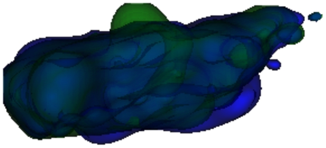
Fig. 9
The initialisation, where the randomly deformed green muscle should return to its initial shape in blue.
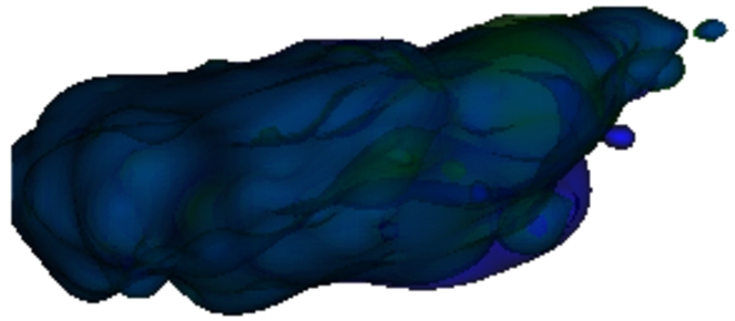
Fig. 10
The restoration copies the original blue shape with the green one, despite minor differences on the right side.
6 Conclusion & Future Work
This paper shows a novel approach for modelling a surface with the radial basis function approach. The proposed method offers a way to model a static and dynamic muscle surface, altogether avoiding recalculating the geometrical model’s parameters to deform it. Even though there are some examples where the approach is not applicable (e.g. the tetrahedron), the suitability for the muscle reconstruction is apparent. Regularisation helps reduce the number of local extrema. However, it also reduces the resulting precision; luckily, a compromise can be reached using a suitable regularisation term selection.
A deformation methodology respecting muscle properties (muscle volume, shape preservation, and bone avoidance) is the most obvious candidate for future work. A good starting point seems to be the work from Cani-Gascuel and Desbrun (
1997) describing the geometrical model deformation in general. However, their method uses the model generated by a skeleton, which is not reasonable for modelling a muscle shape, which would need an overcomplicated skeleton to be able to work. The following work and a great review from Lee
et al. (
2012) describe the possibilities of modelling muscle deformation using skeleton-generated implicit surfaces.
It is not just the novelty but also the oversight of the approach that is apparent; the metric discussed in the article extends beyond its use in muscle modelling or general modelling applications. It is versatile enough to be applied in any situation that requires the comparison of two surfaces. Similarly, the concept of regularisation, with its mathematical underpinnings suitable for RBF surface modelling, can be adapted for broader applications. Its fundamental principle of constraining centres to remain inside applies to more general contexts, such as clustering methodologies.
A Curvature Visualisations
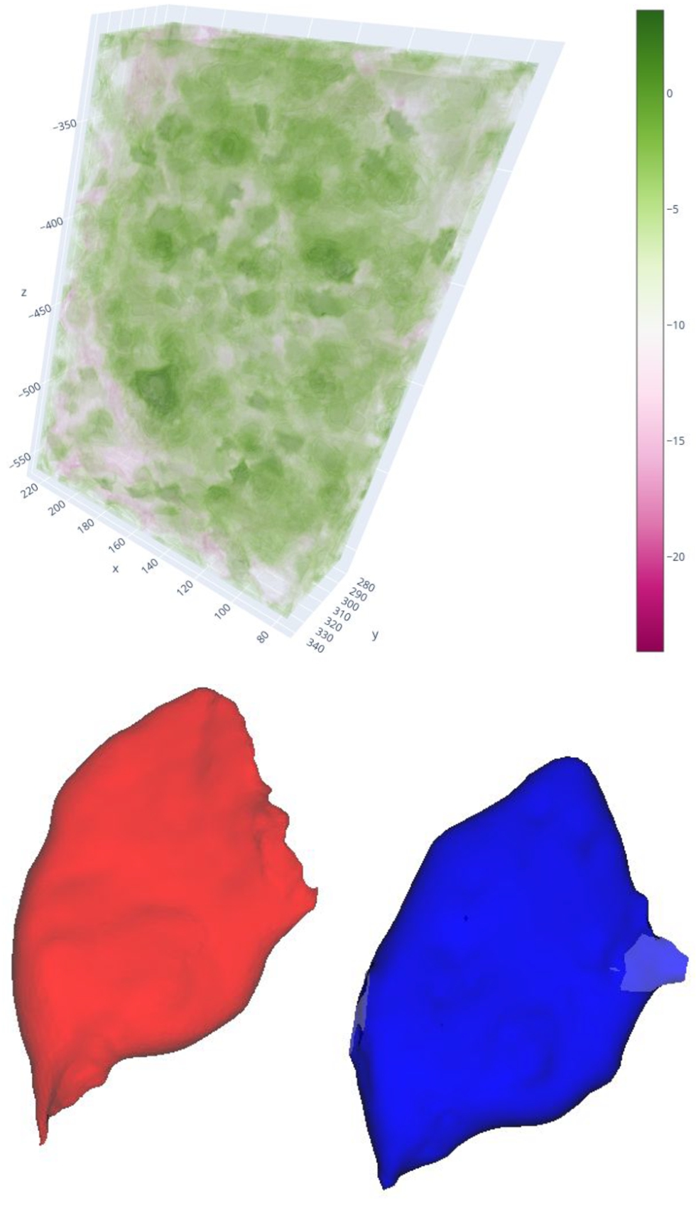
Fig. 11
The curvature of the RBF surface of the gluteus maximus muscle is depicted in the image. The prominent centres of the RBFs are represented by green spheres in the space. The curvature values are displayed in a logarithmic scale, as the differences in curvature are not linear but rather exponential. This result stems from the same experiment shown in Fig.
1; it has been included here for easy comparison.
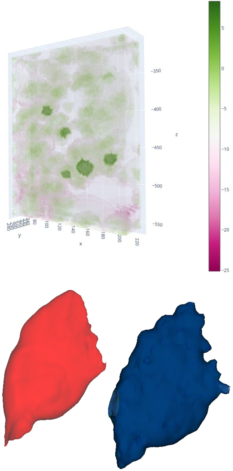
Fig. 12
On the left, we have the curvature field, while on the right, we see the approximation result with a regularisation factor of 0.7. Although there is a preference for curvature fluctuation within the muscle, there is also substantial fluctuation outside. Decreasing the local minima outside the muscle volume results in a less precise approximation of the original red muscle to the blue one.
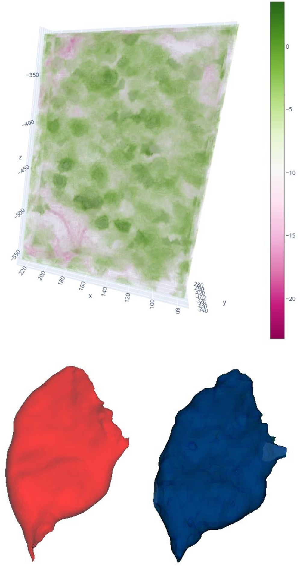
Fig. 13
On the left, we have the curvature field, while on the right, we see the approximation result with a regularisation factor of 0.3. The fluctuation in the curvature field has been further reduced, but as a consequence, the resulting geometrical surface model has become more rough in texture.
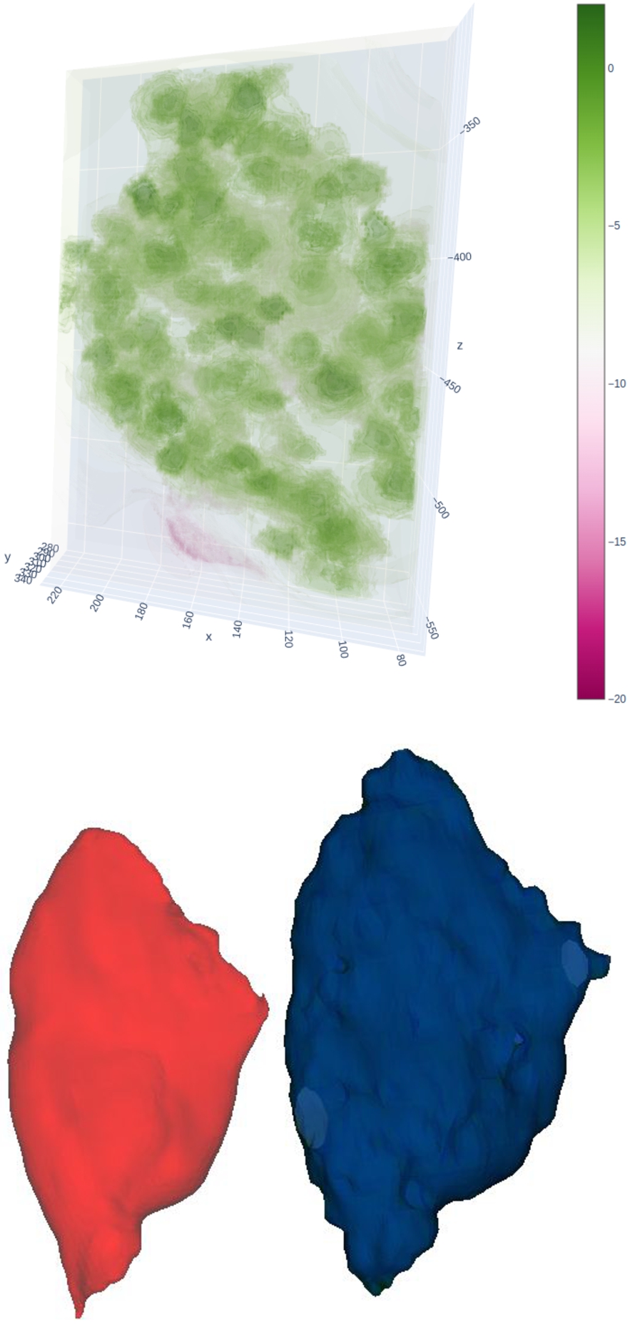
Fig. 14
The curvature field (on the left) and approximation result (on the right) with the regularisation factor of 0.05. While the fluctuation in the curvature field has been nearly eliminated, the roughness of the muscle surface has become quite pronounced.
B Dynamic Restoration Visualisations
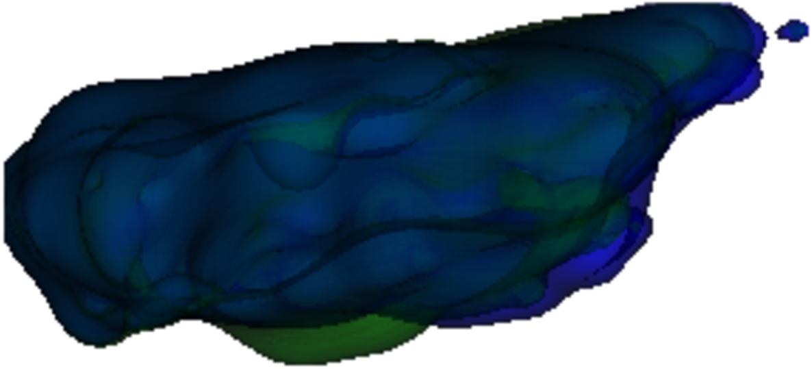
Fig. 15
The initialisation of the simulation without the regularisation factor, where the randomly deformed green muscle should return to its initial shape in blue.
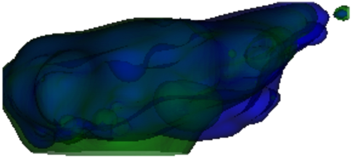
Fig. 16
The progress of the shape restoration. The green surface seems to diverge from the blue one due to omitting the regularisation factor.
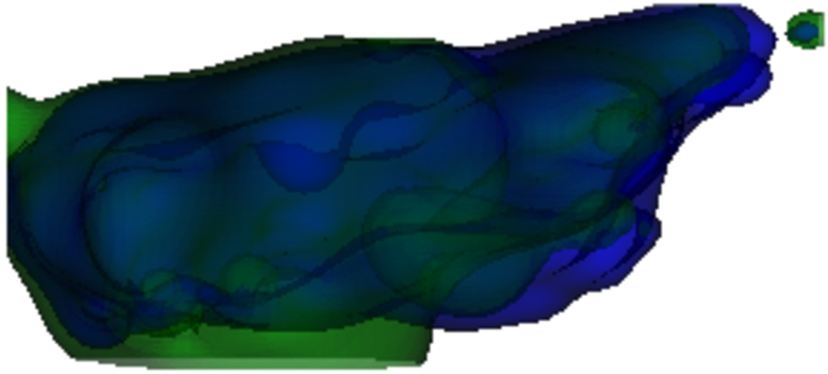
Fig. 17
The final part of the shape restoration. The green shape found other local minima than the muscle’s blue (original) shape.
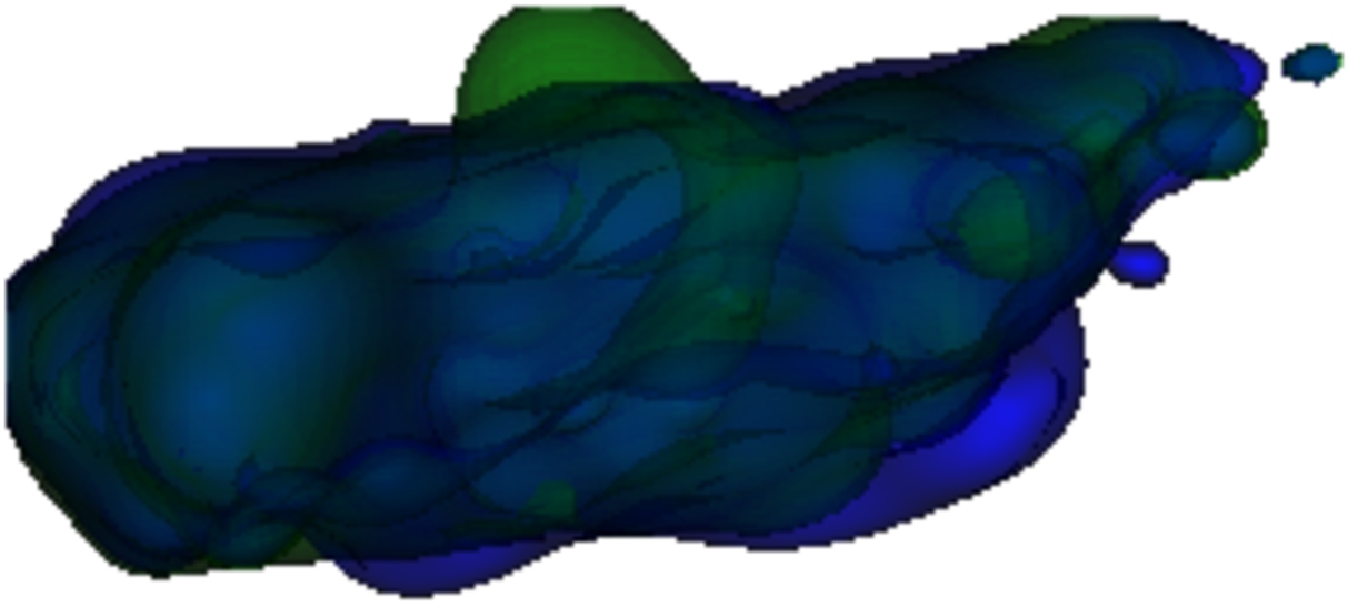
Fig. 18
The initialisation of the simulation with the regularisation factor, where the randomly deformed green muscle should return to its initial shape in blue.
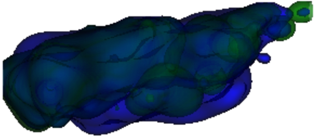
Fig. 19
The green shape seems to converge to the blue shape. The main difference is the restored top part of the green shape.
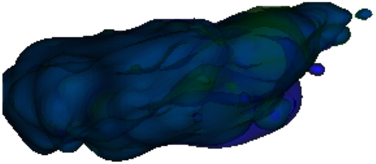
Fig. 20
The final restoration. Excluding the minor differences in the right part of the muscle, the green shape quite accurately approximates the original blue one.
C Mathematical Dynamic Model
Let us assume the function
f to be a 3D radial basis function approximation:
Let’s assume that Gaussian Radial Basis Functions (RBFs) are utilised exclusively. Additionally, we can define
${g_{i}}(\mathbf{x})$ as a replacement for the
ith RBF to streamline subsequent derivations.
The shape of the geometrical model can be well described using its curvature. To compute the curvature, we need to determine the Hessian matrix, consisting of the second partial derivatives with respect to the function
f. Therefore, the initial step involves finding the gradient of the function
f in an
n-dimensional space:
By employing the chain rule, where the expression
$({x_{j}}-{\xi _{ij}})$ originates from the exponent of the exponential function
f, along with the shape parameter
α and the constant value of
$-2$, the resultant gradient takes the following form:
We will now construct the Hessian matrix, which will be used to calculate the curvature. As previously mentioned, its computation relies on knowing the second partial derivatives. In an
nD space, it is defined as follows:
To compute the second partial derivatives, we rely on the gradient of a function
f. For instance, the second partial derivatives with respect to
${x^{2}}$ can be expressed as follows:
Applying the product and chain rules, the second partial derivative with respect to
${x^{2}}$ takes the form of the following expression. The derivation is performed similarly to the first derivative, which has already been carried out above in (
15).
The calculation of the mixed second partial derivatives is performed similarly to before. Upon examining the outcome in (
19), it becomes apparent that there is a resemblance between the mixed partial derivatives and those involving the same variables. The mixed ones are not scaled by
$2{\alpha _{i}}$ and do not undergo a subtraction of 1 from them; otherwise, the remaining operations are identical in both cases.
The Hessian matrix can be populated with the second partial derivatives. Both sets of second partial derivatives involve multiplication by the distances from the centre point in their respective directions. This process can be encapsulated using an outer product. The value of
$-1$ from the pure partial derivatives will transform into the identity matrix with dimensions
$d\times d$, where
d denotes the problem’s dimensionality (which is 3 in our case).
C.1 Mean Curvature
For curvature calculation, one option is to employ the mean curvature, which is defined as the average of all the eigenvalues
${\lambda _{i}}$ of a Hessian matrix:
There are zero eigenvalues with the multiplicity of
$d-1$ and one with a value of
$\| \mathbf{x}-{\boldsymbol{\xi }_{i}}{\| ^{2}}$. The result aligns with the intuition, as zero eigenvalues correspond to eigenvectors perpendicular to the hypersphere isosurface at each point. In contrast, the sole non-zero eigenvalue pertains to the eigenvector tangent to them, pointing from the RBF centre outward. When calculated over the outer product of a vector with itself, the coefficient
$2\alpha $ and identity matrix
${\mathbf{I}_{d}}$ transform the eigenvalues to
$-1$, with a multiplicity of
$d-1$, and the final eigenvalue becomes
$2\alpha \| \mathbf{x}-{\boldsymbol{\xi }_{i}}{\| ^{2}}-1$.
The subsequent step involves specifying the cost function, which is essentially the squared L2 norm between the new and original curvatures across the subspace
$\Omega \subseteq {\mathbb{R}^{d}}$:
One may employ the gradient descent method to discover the optimal values of
${\boldsymbol{\xi }_{i}}$. Initially, we must compute the gradient of the curvature with respect to
${\boldsymbol{\xi }_{i}}$:
The resulting gradient takes the following form:
Now, we need to compute the gradient of the cost function
C, which is expressed as follows:
Given the definition of the partial derivatives of
κ, the complete cost function can be expressed as:
Acknowledgements
The authors thank their colleagues at the University of West Bohemia and the University of Maribor. Thanks to Vaclav Skala and Ivana Kolingerova for their valuable insight and discussion.
Footnotes
References
Abderrazak, K., Benabid, Y. (2022). In: Realistic modeling of shoulder muscle for use in musculoskeletal model. The 13th Conference on Mechanical Engineering CME2022.
Afiatdoust, F., Esmaeilbeigi, M. (2015). Optimal variable shape parameters using genetic algorithm for radial basis function approximation. Ain Shams Engineering Journal, 6(2), 639–647.
https://doi.org/10.1016/j.asej.2014.10.019.
Angles, B., Rebain, D., Macklin, M., Wyvill, B., Barthe, L., Lewis, J., Von Der Pahlen, J., Izadi, S., Valentin, J., Bouaziz, S., Tagliasacchi, A. (2019). VIPER: volume invariant position-based elastic rods. Proceedings of the ACM on Computer Graphics and Interactive Techniques, 2(2) 1–26.
https://doi.org/10.1145/3340260.
Cani-Gascuel, M., Desbrun, M. (1997). Animation of deformable models using implicit surfaces. IEEE Transactions on Visualization and Computer Graphics, 3(1), 39–50.
https://doi.org/10.1109/2945.582343.
Carr, J.C., Beatson, R.K., Cherrie, J.B., Mitchell, T.J., Fright, W.R., McCallum, B.C., Evans, T.R. (2001). Reconstruction and representation of 3D objects with radial basis functions. In: Proceedings of the 28th Annual Conference on Computer Graphics and Interactive Techniques. SIGGRAPH ‘01. Association for Computing Machinery, New York, NY, USA, pp. 67–76.
https://doi.org/10.1145/383259.383266.
Cervenka, M., Smolik, M., Skala, V. (2019). A new strategy for scattered data approximation using radial basis functions respecting points of inflection. In: Misra, S., Gervasi, O., Murgante, B., Stankova, E., Korkhov, V., Torre, C., Rocha, A.M.A.C., Taniar, D., Apduhan, B.O., Tarantino, E. (Eds.), Computational Science and Its Applications – ICCSA 2019. Springer International Publishing, Cham, pp. 322–336.
Cervenka, M., Havlicek, O., Kohout, J., Váša, L. (2023). Computerised muscle modelling and simulation for interactive applications. In: Proceedings of the 18th International Joint Conference on Computer Vision, Imaging and Computer Graphics Theory and Applications (VISIGRAPP 2023) – GRAPP. SciTePress, pp. 214–221.
https://doi.org/10.5220/0011688000003417.
Cieza, A., Causey, K., Kamenov, K., Hanson, S., Chatterji, S., Vos, T. (2020). Global estimates of the need for rehabilitation based on the Global Burden of Disease study 2019: a systematic analysis for the Global Burden of Disease Study 2019. The Lancet, 396(10267), 2006–2017.
https://doi.org/10.1016/S0140-6736(20)32340-0.
Clapés, M., González Hidalgo, M., Torres, A., Palmer-Rodríguez, P. (2008). Interactive constrained deformations of NURBS surfaces: N-SCODEF. In: Articulated Motion and Deformable Objects. AMDO 2008, pp. 359–369.
https://doi.org/10.1007/978-3-540-70517-8_35.
Dvořák, J., Káčereková, Z., Vanecek, P., Hruda, L., Váša, L. (2021). As-rigid-as-possible volume tracking for time-varying surfaces. Computers & Graphics, 102, 329–338.
https://doi.org/10.1016/j.cag.2021.10.015.
Fasser, M., Jokeit, M., Kalthoff, M., Gomez Romero, D.A., Trache, T., Snedeker, J.G., Farshad, M., Widmer, J. (2021). Subject-specific alignment and mass distribution in musculoskeletal models of the lumbar spine. Frontiers in Bioengineering and Biotechnology, 9, 721042.
Goyanes, E., de Moura, J., Fernández-Vigo, J.I., Fernández-Vigo, J.A., Novo, J., Ortega, M. (2024). Automatic simultaneous ciliary muscle segmentation and biomarker extraction in AS-OCT images using deep learning-based approaches. Biomedical Signal Processing and Control, 90, 105851.
https://doi.org/10.1016/j.bspc.2023.105851.
https://www.sciencedirect.com/science/article/pii/S1746809423012843.
Heinrich, D., Bogert, A., Mössner, M., Nachbauer, W. (2023). Model-based estimation of muscle and ACL forces during turning maneuvers in alpine skiing. Scientific Reports, 13, 9026.
https://doi.org/10.1038/s41598-023-35775-4.
Hill, A. (1938). The heat of shortening and the dynamic constants of muscle. Proceedings of the Royal Society of London. Series B, Biological Sciences, 126(843), 136–195.
Hilton, A., Stoddart, A.J., Illingworth, J., Windeatt, T. (1996). Marching triangles: range image fusion for complex object modelling. In: Proceedings of 3rd IEEE International Conference on Image Processing, Vol. 2, pp. 381–3842.
https://doi.org/10.1109/ICIP.1996.560840.
Janák, T., Kohout, J. (2014). Deformable muscle models for motion simulation. In: Proceedings of the 9th International Conference on Computer Graphics Theory and Applications – GRAPP, (VISIGRAPP 2014). SciTePress, pp. 301–311.
https://doi.org/10.5220/0004678903010311.
Joseph, V.R., Hung, Y., Sudjianto, A. (2008). Blind kriging: a new method for developing metamodels. Journal of Mechanical Design, 130(3), 031102.
https://doi.org/10.1115/1.2829873.
Kedadria, A., Benabid, Y., Remil, O., Benaouali, A., May, A., Ramtani, S. (2023). A shoulder musculoskeletal model with three-dimensional complex muscle geometries. Annals of Biomedical Engineering, 51(5), 1079–1093.
https://doi.org/10.1007/s10439-023-03189-y.
Kellnhofer, P., Kohout, J. (2012). Time-convenient deformation of musculoskeletal system. In: Proceedings of ALGORITMY 2012, pp. 1–10.
Kohout, J., Cervenka, M. (2022). Non-planar surface shape reconstruction from a point cloud in the context of muscles attachments estimation. In: Proceedings of the 17th International Joint Conference on Computer Vision, Imaging and Computer Graphics Theory and Applications (VISIGRAPP 2022) – GRAPP. SciTePress, pp. 236–243.
https://doi.org/10.5220/0010869600003124.
Lavoie, P., Ionescu, D., Petriu, E. (2006). Constructing 3D virtual reality objects from 2D images of real objects using NURBS. In: 2007 IEEE Symposium on Virtual Environments, Human-Computer Interfaces and Measurement Systems, Ostuni, Italy, June 25–27, 2007, pp. 117–124.
https://doi.org/10.1109/VECIMS.2007.4373940.
Lee, D., Glueck, M., Khan, A., Fiume, E., Jackson, K. (2012). Modeling and simulation of skeletal muscle for computer graphics: a survey. Foundations and Trends® in Computer Graphics and Vision, 7(4), 229–276.
https://doi.org/10.1561/0600000036.
Lorensen, W.E., Cline, H.E. (1987). Marching cubes: a high resolution 3D surface construction algorithm. ACM SIGGRAPH Computer Graphics, 21(4), pp. 163–169.
https://doi.org/10.1145/37401.37422.
Macklin, M., Müller, M., Chentanez, N. (2016). XPBD: position-based simulation of compliant constrained dynamics. In: Proceedings of the 9th International Conference on Motion in Games. MIG ’16. Association for Computing Machinery, New York, NY, USA, pp. 49–54.
https://doi.org/10.1145/2994258.2994272.
Modenese, L., Renault, J.-B. (2021). Automatic generation of personalized skeletal models of the lower limb from three-dimensional bone geometries. Journal of Biomechanics, 116, 110186.
https://doi.org/10.1016/j.jbiomech.2020.110186.
Ni, N., He, K., Wang, L., Jiang, J., Chen, Z. (2023). Modeling of human muscle and its deformation. Computer Methods in Biomechanics and Biomedical Engineering, 27(3), 365–377.
https://doi.org/10.1080/10255842.2023.2186160.
Nie, M., Wan, Y., Zhou, A. (2022). Real-time NURBS interpolation under multiple constraints. Computational Intelligence and Neuroscience, 2022, 1–15.
https://doi.org/10.1155/2022/7492762.
Oliver, M.A., Webster, R. (1990). Kriging: a method of interpolation for geographical information systems. International Journal of Geographical Information Systems, 4(3), 313–332.
https://doi.org/10.1080/02693799008941549.
Romeo, M., Monteagudo, C., Sánchez-Quirós, D. (2018). Muscle simulation with extended position based dynamics. In: García-Fernández, I., Ureña, C. (Eds.), Spanish Computer Graphics Conference (CEIG). The Eurographics Association, pp. 134–146.
https://doi.org/10.2312/ceig.20181146.
Sakata, S., Ashida, F., Zako, M. (2004). An efficient algorithm for Kriging approximation and optimization with large-scale sampling data. Computer Methods in Applied Mechanics and Engineering, 193(3), 385–404.
https://doi.org/10.1016/j.cma.2003.10.006.
Skala, V. (2017). Least square method robustness of computations: what is not usually considered and taught. In: 2017 Federated Conference on Computer Science and Information Systems, pp. 537–541.
https://doi.org/10.15439/2017F7.
Skala, V., Cervenka, M. (2019). Novel RBF approximation method based on geometrical properties for signal processing with a new RBF function: experimental comparison. In: 2019 IEEE 15th International Scientific Conference on Informatics.
https://doi.org/10.1109/Informatics47936.2019.9119276.
Skala, V., Karim, S.A.A., Zabran, M. (2020). Radial basis function approximation optimal shape parameters estimation. In: Computational Science – ICCS 2020. Springer International Publishing, Cham, pp. 309–317.
Sorkine, O., Alexa, M. (2007). As-rigid-as-possible surface modeling. In: Belyaev, A., Garland, M. (Eds.), Geometry Processing. The Eurographics Association, pp. 109–116.
https://doi.org/10.2312/SGP/SGP07/109-116.
Terzopoulos, D., Qin, H. (1994). Dynamic NURBS with geometric constraints for interactive sculpting. ACM Transactions on Graphics, 13(2), 103–136.
https://doi.org/10.1145/176579.176580.
Valente, G., Martelli, S., Taddei, F., Farinella, G., Viceconti, M. (2012). Muscle discretization affects the loading transferred to bones in lower-limb musculoskeletal models. Proceedings of the Institution of Mechanical Engineers, Part H: Journal of Engineering in Medicine, 226(2), 161–169.
Wang, B., Matcuk, G., Barbič, J. (2021). Modeling of personalized anatomy using plastic strains. ACM Transactions on Graphics, 40(2).
https://doi.org/10.1145/3443703.
Wright, G.B. (2003).
Radial Basis Function Interpolation: Numerical and Analytical Developments. PhD thesis, University of Colorado at Boulder, Boulder, CO, USA. AAI3087597.
Ye, D., Jiang, X., Huo, G., Su, C., Lu, Z., Wang, B., Zheng, Z. (2020). A physical process driven digital terrain model generating method based on D-NURBS. IEEE Access, 8, 3115–3122.
https://doi.org/10.1109/ACCESS.2019.2962385.
Zhang, M., Qin, H. (2001). Hierarchical D-NURBS surfaces and their physics-based sculpting. In: Proceedings International Conference on Shape Modeling and Applications, pp. 257–266.
https://doi.org/10.1109/SMA.2001.923397.
Zhang, Z.-Y., Sun, Z.-J., Yang, Y.-H., Lin, H. (2022). Towards a better prediction of subcellular location of long non-coding RNA. Frontiers of Computer Science, 16(5), 165903.
https://doi.org/10.1007/s11704-021-1015-3.

