1 Introduction
The fuzzy relation (Zadeh, 1971) uses a membership degree to represent the degree that one ordering pair belongs to a relation. Compared with the binary relation, the membership degree of a fuzzy relation belongs to $[0,1]$ rather than the crisp value 0 or 1, which makes the information representation flexible. The fuzzy preference ordering (Tanino, 1984), also called the fuzzy preference relation, was developed to express the fuzzy relations between a set of alternatives. Because fuzzy relations can express experts’ vague information, they have been applied in several realms (Bezdek et al., 1978; Orlovsky, 1978; Fodor and Roubens, 1994; Ferrera-Cedeño et al., 2019; Jin et al., 2020).
Usually, the determination of a fuzzy preference relation requires people to have enough skills in particular aspects. For instance, the fuzzy preference ordering requires people to obey the property of transitivity. The weak transitivity means that, if A is better than B and B is better than C, A should be better than C. Constructing a fuzzy preference ordering needs people to have the perfect ability of computing and inferring data. There are technologies to repair the fuzzy preference ordering which does not obey the transitivity (Saaty, 1977). These technologies force people to make changes on preference information but could not reflect the limited reasoning capacity and knowledge of people. In economic and management realms, the traditional postulate of economic man requires experts to have high or even complete rationality (i.e. the perfect ability of computing and inferring) (Simon, 1955). However, in practice, because of the limitation of human cognition and computation ability, it is difficult for a person to reach the global rationality. To tackle this problem, Simon (1955) proposed the bounded rationality theory, aiming to give a reasonable explanation of human’s real behaviour from the aspects of cognition and psychology. The bounded rationality theory explains rather than restricts human behaviour, and the results of models based on the bounded rationality theory are in line with the real situations of human society (Huang et al., 2013). The bounded rationality theory has also been applied in probability models (Uboe et al., 2017; Le Cadre et al., 2019) and fuzzy decision-making models (Wang and Fu, 2014; Wu and Zhao, 2014; Angus, 2016). The bounded rationality theory does not require people to have a high ability of computing and inferring. Therefore, this paper considers to combine the fuzzy preference relation with the bounded rationality theory. Given that the development of a fuzzy preference relation was based on four properties including reflexivity, symmetry, transitivity, and reciprocity (which will be explained in detail in Section 2), we need to investigate whether the four properties are in line with the bounded rationality theory.
In this study, the usability of the four properties of a fuzzy preference relation is firstly discussed under the bounded rationality situation. It is found that all four properties do not satisfy the bounded rationality. Because the transitivity might be violated in real decision-making problems (Świtalski, 2001) and it is a problem to select a suitable definition of transitivity from a group of definitions of transitivity (Zadeh, 1971; Wang, 1997; Herrera-Viedma et al., 2004), we try to improve the definition of reciprocity. Then, a new property called the bounded rational reciprocity is proposed. Based on the new property, the bounded rational reciprocal preference relation is introduced. A rationality visualization technique and a bounded rationality net-flow-based ranking method are presented to help people apply the bounded rational reciprocal preference relation to solve real decision-making problems.
The contributions of this study are highlighted as follows:
-
(1) We introduce the bounded rational reciprocity. Since the reflexivity, symmetry, transitivity, and reciprocity do not suit the bounded rationality theory, we propose the rationality value to define a new property called the bounded rational reciprocity. Compared with the transitivity and reciprocity, the bounded rational reciprocity explains rather than restricts the membership degree, which reduces the difficulty of collecting information and improves the flexibility of decision making.
-
(2) The bounded rational reciprocal preference relation is proposed to model the limited ability of people. By combining the idea of the bounded rational reciprocity and fuzzy preference relation, we introduce the bounded rational reciprocal preference relation. The rationality radius is presented to explain experts’ rationality. The rationality visualization technique is introduced to intuitively display the rationality of experts.
-
(3) A bounded rationality net-flow-based method is presented to rank alternatives in decision-making problems. With the weights of experts, the aggregated bounded rational reciprocal preference relation is calculated. The positive and negative bounded rationality flow is introduced to get the bounded rationality net flow, which can be further used to rank alternatives. A numerical example is given to demonstrate the bounded rationality net-flow-based decision-making method. Comparative analyses with the reciprocal preference relation and non-reciprocal preference relation are given to show the advantages of the proposed decision-making method.
This study is organized as follows: In Section 2, we review the bounded rationality theory and fuzzy preference relation. In Section 3, the bounded rational reciprocity and bounded rational reciprocal preference relation are proposed. Section 4 introduces the rationality visualization technique and the bounded rationality net-flow-based ranking method. A numerical example is also given in Section 4. Section 5 closes the paper with concluding remarks.
2 Preliminaries
For the convenience of presentation, in this section, the relevant theories are introduced.
2.1 Fuzzy Relation and Its Developments
To analyse the incompatibility between fuzzy preference relations and the bounded rationality, this section introduces the fuzzy preference relation and its developments. We begin with the concept of binary relation.
For two sets of evaluations on alternatives x and y, $X=\{{x_{1}},{x_{2}},\dots \}$ and $Y=\{{y_{1}},{y_{2}},\dots \}$, the product set $X\times Y$ is $\{({x_{i}},{y_{\xi }})|{x_{i}}\in X,{y_{\xi }}\in Y\}$, where $({x_{i}},{y_{\xi }})$ is an ordering pair. Any subset of $X\times Y$ is a binary relation. For a fixed relation “R”, if an ordering pair $({x_{i}},{y_{\xi }})$ belongs to the relation “R”, alternative ${x_{i}}$ is regarded to have a relation “R” with alternative ${y_{\xi }}$. Given a set of two supply chain suppliers $X=\{{x_{1}},{x_{2}}\}$, the product set $X\times X$ is $\{({x_{1}},{x_{1}}),({x_{1}},{x_{2}}),({x_{2}},{x_{1}}),({x_{2}},{x_{2}})\}$. Let the binary relation “R” be “better”. If the supplier ${x_{1}}$ is better than the supplier ${x_{2}}$, then the ordering pair $({x_{1}},{x_{2}})$ belongs to the relation “R”. Likewise, if the ordering pair $({x_{1}},{x_{2}})$ belongs to the relation “R”, it means that the supplier ${x_{1}}$ is better than the supplier ${x_{2}}$.
In the above Example 1, if we know that ${x_{1}}$ is better than ${x_{2}}$, it can be inferred that the ordering pair $({x_{1}},{x_{2}})$ must belong to “R”. However, because of the complexity of practical management activities, ${x_{1}}$ is usually partly better than ${x_{2}}$. In this situation, we cannot say that the ordering pair $({x_{1}},{x_{2}})$ totally belongs to “R”. To model such situations, Zadeh (1971) used the fuzzy theory to define the fuzzy relation (or fuzzy binary relation) where the degree of $({x_{i}},{y_{\xi }})$ belonging to the relation “R” was a membership degree ${\mu _{R}}({x_{i}},{y_{\xi }})\in [0,1]$. Particularly, when ${\mu _{R}}({x_{i}},{y_{\xi }})$ is 0, $({x_{i}},{y_{\xi }})$ does not belong to “R”; when ${\mu _{R}}({x_{i}},{y_{\xi }})$ is 1, $({x_{i}},{y_{\xi }})$ belongs to “R”. In other words, the binary relation is a special case of the fuzzy relation where the membership degree ${\mu _{R}}({x_{i}},{y_{\xi }})$ is 0 or 1.
For fuzzy relations, they have four properties, namely, reflexivity, symmetry, transitivity, and reciprocity (Zadeh, 1971; Bezdek et al., 1978). The reflexivity means ${\mu _{R}}({x_{i}},{x_{i}})=1$, which is related to the partial ordering. If ${\mu _{R}}({x_{i}},{x_{i}})=0$, the partial ordering could not be set up. The symmetry means ${\mu _{R}}({x_{i}},{y_{\xi }})={\mu _{R}}({y_{\xi }},{x_{i}})$. There is a mass of rules of the transitivity, satisfying different requirements in different situations (Wang, 1997; Herrera-Viedma et al., 2004; Chang et al., 2019). The main role of transitivity is to avoid the inconsistency that might cause errors and paradoxes. The reciprocity is ${\mu _{R}}({x_{i}},{y_{\xi }})+{\mu _{R}}({y_{\xi }},{x_{i}})=1$ $({x_{i}}\ne {y_{\xi }})$, meaning that the degree of ${x_{i}}$ dominating ${y_{\xi }}$ plus the degree of ${y_{\xi }}$ dominating ${x_{i}}$ must be 1.
Different combinations of these four properties yielded different developments of the fuzzy relation. These developments could be divided into two categories. Regarding the first group, Zadeh (1971) proposed a few concepts which mainly focused on transitivity, symmetry, and reflexivity. The fuzzy ordering was the fuzzy relation having transitivity. The fuzzy preordering was the fuzzy ordering having reflexivity. The similarity relation was the fuzzy preordering satisfying the symmetry. The fuzzy partial ordering was the fuzzy preordering which was anti-symmetric. The fuzzy linear ordering was the fuzzy partial ordering satisfying ${x_{i}}\ne {y_{\xi }}\Rightarrow {\mu _{R}}({x_{i}},{y_{\xi }})>0$ or ${\mu _{R}}({y_{\xi }},{x_{i}})>0$. The fuzzy weak ordering was the fuzzy preordering having ${x_{i}}\ne {y_{\xi }}\Rightarrow {\mu _{R}}({x_{i}},{y_{\xi }})>0$ or ${\mu _{R}}({y_{\xi }},{x_{i}})>0$. In the second group, the reciprocity and the necessity of transitivity were investigated. Bezdek et al. (1978) proposed the reciprocal property and defined the reciprocal fuzzy relation which was irreflexive and reciprocal. Orlovsky (1978) proposed the fuzzy non-strict preference relation which was a reflexive but not necessarily a transitive fuzzy relation. Tanino (1984) introduced the fuzzy preference ordering which was reciprocal and transitive. Based on the fuzzy non-strict preference relation, Parreiras et al. (2012) defined the nonreciprocal property and introduced a nonreciprocal fuzzy preference relation. Motivated by Nakamura (1986), we give Fig. 1 to clearly illustrate the relations of these developments of the fuzzy relation.
Among the developments of fuzzy relations, the fuzzy preference ordering attracted the attention of many researchers. Different kinds of uncertainty were considered to improve the fuzzy preference ordering. Xu (2007) proposed the intuitionistic preference relation considering the membership and non-membership degrees. Liao et al. (2014) introduced the hesitant fuzzy preference relation which could express experts’ hesitancy degrees. There were triangular fuzzy reciprocal preference relation (Meng et al., 2017) in which the membership function was a triangular fuzzy number and interval fuzzy preference relation (Meng et al., 2019) using intervals to express uncertainty. Zhang et al. (2019) presented the q-rung orthopair fuzzy preference relation to deal with the problems that the membership degree plus non-membership degree is larger than 1. Gong et al. (2020) proposed the linear uncertain preference relation. The use of fuzzy relations in decision making facilitated its developments in theory (Wan et al., 2017; Ferrera-Cedeño et al., 2019; Zhang et al., 2021). Known from Section 2.2., experts are usually bounded rational. However, as far as we know, few studies discussed the suitability of the four properties within the context of bounded rationality.
2.2 Bounded Rationality Theory
In the traditional economic theory, there is a postulate of economic man, that experts are familiar with, who has related knowledge and a stable system of preference (Simon, 1955). This economic man postulate requires experts to have high rationality, and thus it is also called the global rationality postulate (Simon, 1955). The postulate of economic man simplifies the analysis of real problems by mathematical models. In real situations, especially in economic and management realms, practical issues might be complex. Usually, an expert is only proficient in one or two areas. Facing practical issues that involve many areas like the law and marketing, experts might not have enough knowledge, which causes the cognitive limitation of experts. Besides, experts’ computation ability is limited. When there is a large amount of data, experts might not be able to process the whole data, resulting in the weak estimation of the result of a decision. Because the cognition levels of experts are limited by their knowledge, it is hard for them to satisfy the global rationality postulate. In this situation, the simplification of real problems by the postulate of economic man might cause unreasonable results.
To make the postulate of economic man compatible with experts’ abilities, Simon (1955) first proposed the concept of bounded rationality. Different from the global rationality postulate which restricts human behaviours, the bounded rationality theory aims to give a reasonable explanation for experts’ realistic behaviours from the aspects of human cognition and psychology. To achieve this goal, decision processes and methods were simplified from the perspective of the gross characteristics of human choice (Simon, 1955) and the broad features of the environment (Simon, 1956). A few interesting notions, such as the satisfactory solutions (Simon, 1955), were proposed based on the bounded rationality theory.
Motivated by the bounded rationality theory, a mass of researches has been done, which can be grouped into two categories. The first group considered probability models with the bounded rationality theory. Mattsson and Weibull (2002) reviewed the development of the game theory with the bounded rationality and proposed a probabilistic choice model with bounded rationality. Sterman et al. (2007) combined the bounded rationality theory with disequilibrium dynamics to create a dynamic behavioural game model. Huang et al. (2013) used a special queue model, where customers’ waiting time cannot be accurately estimated, to capture the bounded rationality, and concluded that if the bounded rationality was ignored, there was a “significant revenue and welfare loss”. The second group focused on the fuzzy theory. Angus (2016) found that, in addition to the probability theory, it was also necessary to consider the fuzzy theory together with the bounded rationality theory. Wang and Fu (2014) used a nonlinear scalarization technique to model bounded rationality in generalized abstract fuzzy economies. Wu and Zhao (2014) proposed the fuzzy choice functions of fuzzy preference relations under the circumstance of bounded rationality. Chang et al. (2019) considered the transitivity of fuzzy preference relations with bounded rationality and proposed the triangular bounded consistency of fuzzy preference relations. Furthermore, the bounded rationality theory has achieved several applications in terms of organization management (Simon, 1991), transportation system design (Cascetta et al., 2015), stock management (Sterman, 1989), policy advice (Caballero and Lunday, 2020), hotel selection (Wang et al., 2020), and the analysis of customers’ behaviours in service operations systems (He et al., 2020).
For the existing researches on fuzzy preference relations under the bounded rationality circumstance (Wang and Fu, 2014; Wu and Zhao, 2014), the core idea was to use formulas and constraints to express the bounded rationality, which was similar to Lipman’s idea (1991). However, they ignored a key problem that the original properties of fuzzy preference relations might not be compatible with the bounded rationality. This incompatibility might cause systematic and inherent errors when using existing methods (Wang and Fu, 2014; Wu and Zhao, 2014). In Section 3, we will further analyse this incompatibility in detail.
3 Bounded Rational Reciprocal Preference Relation
As mentioned in Section 2.1, few studies investigated the four properties of fuzzy relations within the context of bounded rationality. If the four properties are not compatible with the bounded rationality theory, the applications of fuzzy relations might be limited in practice. In this section, we begin with the discussion on the question whether the four properties are compatible with the bounded rationality. It is found that all four properties do not satisfy the bounded rationality theory. Thus, a new property called the bounded rational reciprocity is proposed. Then, the bounded rational reciprocal preference relation is introduced based on the bounded rational reciprocity.
3.1 Whether the Properties of Fuzzy Relation are in Line with the Bounded Rationality Theory?
Different relations “R” have different rules of reflexivity. When the relation “R” is “equal or better”, the reflexivity can be ${\mu _{R}}({x_{i}},{x_{i}})=1$ (Zadeh, 1971) and ${\mu _{R}}({x_{i}},{x_{i}})=0.5$ (Tanino, 1984). When the relation “R” is “better”, the reflexivity can be ${\mu _{R}}({x_{i}},{x_{i}})=0$ (Bezdek et al., 1978). In complex decision-making problems, the relations “equal or better” and “better” given by experts are approximate relations. When ${x_{i}}$ and ${x_{j}}$ represent organizations or experts, it is hard to strictly determine the relation between ${x_{i}}$ and ${x_{j}}$ due to their cognitive limitation. For instance, when experts give the information that company A is better than company B, the relation “better” is an approximate relation because it is ill-defined. If experts are asked to strictly determine the approximate relation “better”, they should have high rationalities. In this high rationality situation, it is difficult to select the rules of reflexivity under bounded rationality theory.
The symmetry means that the membership degree of ${x_{i}}$ being better than ${x_{j}}$ is the same as that of ${x_{j}}$ being better than ${x_{i}}$ (Zadeh, 1971). Different from the symmetry, the reciprocity requires that ${\mu _{R}}({x_{i}},{x_{j}})$ plus ${\mu _{R}}({x_{j}},{x_{i}})$ is 1 (Bezdek et al., 1978). Because these two properties require experts to give information in special constraints like ${\mu _{R}}({x_{i}},{x_{j}})={\mu _{R}}({x_{j}},{x_{i}})$ or ${\mu _{R}}({x_{i}},{x_{j}})+{\mu _{R}}({x_{j}},{x_{i}})=1$, the experts must have enough knowledge and high cognitive level to provide accurate information. In other words, the experts should be rational, which goes against the bounded rationality theory.
There is a mass of rules concerning transitivity which requires experts to have a stable preference system (Zadeh, 1971; Wang, 1997; Herrera-Viedma et al., 2004; Chang et al., 2019). On one hand, an empirical study has pointed out that experts’ preferences might violate the transitivity (Świtalski, 2001), so the transitivity might not be necessary. On the other hand, different experts might have different reasoning processes, so the fixed transitivity might restrict experts’ behaviours. This restriction is also not in line with the bounded rationality theory.
3.2 Bounded Rational Reciprocal Preference Relation with the Bounded Rational Reciprocity
According to the analyses in Section 3.1, it is clear that the four properties are not compatible with the idea of the bounded rationality theory. Motivated by the idea of the reciprocal index (Dong et al., 2008), we propose a new property satisfying bounded rationality.
Most of the time, ${\mu _{R}}({x_{i}},{x_{j}})$ is not the same as ${\mu _{R}}({x_{j}},{x_{i}})$, so the symmetry is not considered. For reflexivity and transitivity, there are a mass of rules, but the fixed rules might restrict human behaviour. Hence, we do not consider reflexivity and transitivity. For the reciprocity, the “1” on the right side of ${\mu _{R}}({x_{i}},{x_{j}})+{\mu _{R}}({x_{j}},{x_{i}})=1$ is the limitation. When experts’ knowledge is not enough, they cannot clearly judge ${\mu _{R}}({x_{i}},{x_{j}})$ and ${\mu _{R}}({x_{j}},{x_{i}})$. If they are conservative, ${\mu _{R}}({x_{i}},{x_{j}})+{\mu _{R}}({x_{j}},{x_{i}})$ might be smaller than 1. If not, when experts’ cognitive level is low, there might be a high intersection between ${\mu _{R}}({x_{i}},{x_{j}})$ and ${\mu _{R}}({x_{j}},{x_{i}})$, resulting in ${\mu _{R}}({x_{i}},{x_{j}})+{\mu _{R}}({x_{j}},{x_{i}})>1$. Based on this idea, we replace “1” with a value τ to demonstrate an expert’s rationality level. Then, the bounded rational reciprocity is defined as follows:
Note. The relation R in the bounded rational reciprocity can be “equal or better” or “better”. There is no strict requirement on R.
Definition 1.
For two alternatives ${x_{i}}$ and ${x_{j}}$ in $X=\{{x_{1}},{x_{2}},\dots ,{x_{n}}\}$, the membership degree of the ordering pair (${x_{i}},{x_{j}}$) belonging to the relation “R” is ${\mu _{R}}({x_{i}},{x_{j}})$, abbreviated as ${\mu _{ij}}$. The bounded rational reciprocity is given as ${\mu _{ij}}+{\mu _{ji}}={\tau _{ij}}$, where ${\tau _{ij}}={\tau _{ji}}$ is the rationality value of the expert regarding the relation “R” of ${x_{i}}$ and ${x_{j}}$.
For a fuzzy relation, the membership degree ${\mu _{ij}}$ belongs to [0, 1]. Hence, ${\tau _{ij}}$ belongs to $[0,2]$. When the rationality of an expert is low, the knowledge reserve is insufficient and the cognitive level is low, causing ${\tau _{ij}}$ to deviate from 1. Hence, when $|{\tau _{ij}}-1|$ is large, the rationality of the expert is low, which means that the expert has a poor understanding of ${x_{i}}$ and ${x_{j}}$. This indicates that the membership degrees ${\mu _{ij}}$ and ${\mu _{ji}}$ are unreliable. It is noticed that ${\tau _{ij}}=1$ does not mean that the expert is totally rational.
Transitivity was usually used to judge experts’ rationality. If the preference did not satisfy the transitivity, some consistency adjustment methods (Herrera-Viedma et al., 2004; Jin et al., 2020) were proposed to modify the given preference information. These studies held the view that the preference dissatisfying the transitivity was irrational, so the change was necessary. However, experts might have their special transitivity property even though their preference information does not satisfy certain transitivity. In other words, this does not mean that the experts are irrational (Karapetrovic and Rosenbloom, 1999).
Compared with the transitivity and reciprocity, the bounded rational reciprocity tries to explain rather than restrict membership degrees. As the bounded rational reciprocity does not limit the value of ${\mu _{ij}}+{\mu _{ji}}$, experts can give information with freedom. This reduces the difficulty of collecting information. In this sense, the bounded rational reciprocity is meaningful to the decision-making theory.
Because the reflexivity, symmetry, transitivity and reciprocity do not satisfy the bounded rationality, the existing preference relations reviewed in Section 2.2 are not compatible with the bounded rationality theory. Because the bounded rational reciprocity, which is in line with the bounded rationality theory, has superiorities in decision making, we propose the bounded rational reciprocal preference relation based on the bounded rational reciprocity.
Definition 2.
For a given alternative set $X=\{{x_{1}},{x_{2}},\dots ,{x_{n}}\}$, the bounded rational reciprocal preference relation is the fuzzy relation $\mu :X\times X\to [0,1]$, satisfying the bounded rational reciprocity that ${\mu _{ij}}+{\mu _{ji}}={\tau _{ij}}$ $(\forall {x_{i}},{x_{j}}\in X,{x_{i}}\ne {x_{j}})$ where ${\tau _{ij}}\in [0,2]$.
The bounded rational reciprocal preference relation on an alternative set $X=\{{x_{1}},{x_{2}},\dots ,{x_{n}}\}$ can be expressed as a matrix $B={[{\mu _{ij}}]_{n\times n}}$ $(\forall {x_{i}},{x_{j}}\in X,{x_{i}}\ne {x_{j}})\in X\times X$ where ${\mu _{ij}}\in [0,1]$ and ${\mu _{ij}}+{\mu _{ji}}={\tau _{ij}}$ (${\tau _{ij}}\in [0,2]$).
In practical decision-making processes, experts may have different understandings about different alternatives, causing various ${\tau _{ij}}$. Here, we can define a rationality radius $r=\{\min \varepsilon |\forall {x_{i}},{x_{j}}\in X,{\tau _{ij}}\in [1-\varepsilon ,1+\varepsilon ]\}$. $[1-r,1+r]$ is the smallest interval involving all rationality values. The rationality radius can be calculated as $r={\max _{i\ne j}}\{|{\tau _{ij}}-1|\}$. Because ${\tau _{ij}}\in [0,2]$, we have $r\in [0,1]$. The high rationality radius indicates low rationality on all alternatives in X.
Example 1.
For a given alternative set $X=\{{x_{1}},{x_{2}},{x_{3}}\}$, the membership degrees might be ${\mu _{1,2}}=0.2$, ${\mu _{2,1}}=0.9$, ${\mu _{1,3}}=0.5$, ${\mu _{3,1}}=0.7$, ${\mu _{2,3}}=0.4$, and ${\mu _{3,2}}=0.3$. ${\mu _{1,3}}=0.5$ means that the degree of ${x_{1}}$ dominating ${x_{3}}$ is 0.5. The matrix of the bounded rational reciprocal preference relation is
The rationality radius is $\max \{0.1,0.2,0.3\}=0.3$.
The developments of fuzzy relations based on the reciprocity, like the fuzzy preference ordering (Tanino, 1984), cannot express the data in Example 1. Because the bounded rational reciprocal preference relation does not have the constrain ${\mu _{ij}}+{\mu _{ji}}=1$, it can express the preference information in Example 1. Since experts can give membership degrees without the constrain ${\mu _{ij}}+{\mu _{ji}}=1$, the convenience of giving information is enhanced. These two merits show that the bounded rational reciprocal preference relation is significant for decision making.
3.3 A Rationality Visualization Technique to Display the Rationality of Experts
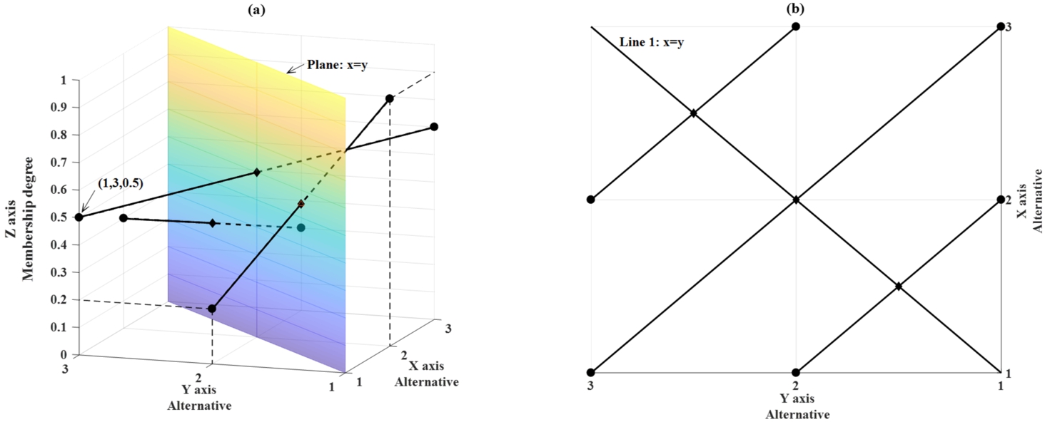
The membership degrees in the bounded rational reciprocal preference relation can be represented by the triples $(i,j,{\mu _{ij}})$, where $i,j=1,2,\dots ,n$ $(i\ne j)$. Then, these triples can be marked in a 3D coordinate system where the X and Y axes represent the subscripts of the elements in the alternative set $X=\{{x_{1}},{x_{2}},\dots ,{x_{n}}\}$, and the Z axis represents membership degrees.
For all pairs $(i,j,{\mu _{ij}})$ and $(j,i,{\mu _{ji}})$ $(i,j=1,2,\dots ,n,\hspace{2.5pt}i\ne j)$, the midpoints of their connecting lines are ($(i+j)/2,(i+j)/2,({\mu _{ij}}+{\mu _{ji}})/2$). This indicates that all midpoints are on the $x=y$ plane. It is explained in Section 3.2 that the distance between ${\tau _{ij}}$ and 1 shows the rationality level. Thus, the distance between $({\mu _{ij}}+{\mu _{ji}})/2={\tau _{ij}}/2$ and 0.5 can show the rationality level. Hence, we let the midpoints ($(i+j)/2,(i+j)/2,{\tau _{ij}}/2$) ($i,j=1,2,\dots ,n,\hspace{2.5pt}i\ne j$) be the rationality points.
However, in the 3D coordinate system, the midpoints are not easy to be visually distinguished, so it is necessary to make a transformation. Let ${t_{ij}}=\sqrt{2}\times (i+j)/2$. Then, the transformed rationality points are (${t_{ij}},{\tau _{ij}}/2$) $(i,j=1,2,\dots ,n,\hspace{2.5pt}i\ne j)$, which can be marked in a 2D coordinate system. This 2D coordinate system is called the rationality plane, where two axes represent membership degrees and ${t_{ij}}$, respectively.
Example 2.
Fig. 2
The 3D coordinate system of the bounded rational reciprocal preference relation in Example 2.
In Fig. 2(a), there is a point which represents that the membership degree of $({x_{1}},{x_{3}})$ belonging to the relation R is 0.5. Fig. 2(b) is a projection of Fig. 2(a) on the $X-Y$ plane. Line 1 in Fig. 2(b) is the projection of the $x=y$ plane. The rationality points can be calculated as $(1.5,1.5,0.55)$, $(2,2,0.6)$, and $(2.5,2.5,0.35)$, which are marked out as rhombuses in Fig. 2. The transformed rationality points are $(3\sqrt{2}/2,0.55)$, $(2\sqrt{2},0.6)$, and $(5\sqrt{2}/2,0.35)$. The rationality chart is shown in Fig. 3. The rationality radius is the distance between the two dotted lines in Fig. 3. The closer the transformed rationality points get to the centreline, the more rational the experts are. From Fig. 2(b) and Fig. 3, it is easy to find that the T axis in Fig. 3 is the line $x=y$ in Fig. 2(b). The rationality chart illustrates the $x=y$ plane in Fig. 2(a).
4 Decision Making Based on the Bounded Rational Reciprocal Preference Relation
To use the bounded rational reciprocal preference relation in order to solve decision-making problems, we propose a bounded rationality net-flow-based method to rank alternatives.
4.1 A Bounded Rationality Net-Flow-Based Ranking Method for Decision Making
Before proposing the bounded rationality net-flow-based ranking method, we first make a description of the decision making framework. There are n alternatives denoted by $X=\{{x_{1}},{x_{2}},\dots ,{x_{n}}\}$ to be ranked. k experts $P=\{{p^{1}},{p^{2}},\dots ,{p^{k}}\}$ provide the preference information of the alternatives by a bounded rational reciprocal preference relation ${B^{k}}={[{\mu _{ij}^{k}}]_{n\times n}}$ ($\forall {x_{i}},{x_{j}}\in X,\hspace{2.5pt}{x_{i}}\ne {x_{j}}$). The membership degree ${\mu _{ij}^{k}}$ belonging to [$0,1$] shows the degree of ${x_{i}}$ preferred to ${x_{j}}$. ${\mu _{ij}^{k}}=0$ means ${x_{i}}$ is not preferred to ${x_{j}}$ while ${\mu _{ij}^{k}}=1$ means ${x_{i}}$ is completely preferred to ${x_{j}}$. The problem is to rank the alternatives according to the bounded rational reciprocal preference relation.
If the rationality of expert ${p^{k}}$ is high, the preference information ${B^{k}}$ is reliable. Hence, when we integrate the preference information of all experts, the experts with high rationality should have high weights. For expert ${p^{k}}$, if the average of the rationality values is close to 1, the expert is rational. If the rationality radius is small, the expert has good understanding on each alternative. Considering these two aspects, the weight of the expert ${p^{k}}$ can be calculated as:
where ${\eta ^{k}}={e^{-(|2\times {\textstyle\sum _{i<j}}{\tau _{ij}^{k}}/(n\times (n-1))-1|+{r^{k}})}}$. ${\tau _{ij}^{k}}={\mu _{ij}^{k}}+{\mu _{ji}^{k}}$ is the rationality value of alternatives ${x_{i}}$ over ${x_{j}}$ corresponding to expert ${p^{k}}$. ${r^{k}}$ is the rationality radius of ${B^{k}}$.
Then, k bounded rational reciprocal preference relations can be aggregated to an aggregated bounded rational reciprocal preference relation ${B^{A}}={({\mu _{ij}})_{n\times n}}$ ($\forall {x_{i}},{x_{j}}\in X,\hspace{2.5pt}{x_{i}}\ne {x_{j}}$), where ${\mu _{ij}}={\textstyle\sum _{k}}{w^{k}}\times {\mu _{ij}^{k}}$.
For alternatives ${x_{i}}$ and ${x_{j}}$, if the rationality value ${\tau _{ij}}$ is close to 1, the membership degrees ${\mu _{ij}}$ and ${\mu _{ji}}$ are reliable. Hence, the weights of alternative pairs ${x_{i}}$ and ${x_{j}}$ are
where ${\theta _{ij}}={e^{-|{\tau _{ij}}-1|}}$. ${\tau _{ij}}={\mu _{ij}}+{\mu _{ji}}$. Because ${\tau _{ij}}={\tau _{ji}}$, ${w_{ij}}={w_{ji}}$.
(2)
\[ {w_{ij}}=\frac{{\theta _{ij}}}{{\textstyle\sum _{i}}{\textstyle\sum _{j>i}}{\theta _{ij}}},\]For an alternative ${x_{i}}$, ${\textstyle\sum _{j\ne i}}{w_{ij}}\times {\mu _{ij}}$ can be seen as the weighted sum of the degree of ${x_{i}}$ dominating other alternatives. On the contrary, ${\textstyle\sum _{j\ne i}}{w_{ji}}\times {\mu _{ji}}$ can be seen as the weighted sum of the degree of other alternatives dominating ${x_{i}}$. Let ${\textstyle\sum _{j\ne i}}{w_{ij}}\times {\mu _{ij}}$ and ${\textstyle\sum _{j\ne i}}{w_{ji}}\times {\mu _{ji}}$ be the positive bounded rationality flow ${S_{i}^{+}}$ and negative bounded rationality flow ${S_{i}^{-}}$ of ${x_{i}}$. The bounded rationality net flow of ${x_{i}}$ is
where ${w_{ij}}={w_{ji}}$. The high bounded rationality net flow ${S_{i}}$ indicates that ${x_{i}}$ has a good performance. Hence, we can rank alternatives in descending order of the bounded rationality net flow.
(3)
\[ {S_{i}}=\sum \limits_{j\ne i}{w_{ij}}\times {\mu _{ij}}-\sum \limits_{j\ne i}{w_{ji}}\times {\mu _{ji}},\]Proof.
For any ${\mu _{ij}}$, its sign is a positive sign in ${S_{i}}$, and its sign is negative in ${S_{j}}$. Because ${w_{ij}}={w_{ji}}$, the contribution of ${\mu _{ij}}$ to ${\textstyle\sum _{i}}{S_{i}}$ is ${w_{ij}}\times {\mu _{ij}}-{w_{ji}}\times {\mu _{ij}}=0$. Thus, it can be inferred that ${\textstyle\sum _{i}}{S_{i}}=0$. □
4.2 A Numerical Example
This section gives a numerical example to illustrate the bounded rationality net-flow-based ranking method. Suppose that three experts $P=\{{p^{1}},{p^{2}},{p^{3}}\}$ are asked to assess three alternatives $X=\{{x_{1}},{x_{2}},{x_{3}}\}$ with bounded rational preference relations, shown as follows:
\[\begin{aligned}{}& {B^{1}}=\left[\begin{array}{c@{\hskip4.0pt}c@{\hskip4.0pt}c}\setminus \hspace{1em}& 0.5\hspace{1em}& 0.6\\ {} 0.6\hspace{1em}& \setminus \hspace{1em}& 0.3\\ {} 0.3\hspace{1em}& 0.7\hspace{1em}& \setminus \end{array}\right],\hspace{2em}{B^{2}}=\left[\begin{array}{c@{\hskip4.0pt}c@{\hskip4.0pt}c}\setminus \hspace{1em}& 0.2\hspace{1em}& 0.3\\ {} 0.6\hspace{1em}& \setminus \hspace{1em}& 0.7\\ {} 0.8\hspace{1em}& 0.5\hspace{1em}& \setminus \end{array}\right],\\ {} & {B^{3}}=\left[\begin{array}{c@{\hskip4.0pt}c@{\hskip4.0pt}c}\setminus \hspace{1em}& 0.6\hspace{1em}& 0.3\\ {} 0.5\hspace{1em}& \setminus \hspace{1em}& 0.8\\ {} 0.7\hspace{1em}& 0.3\hspace{1em}& \setminus \end{array}\right].\end{aligned}\]
In ${B^{1}}$, 0.5 means that the alternative ${x_{1}}$ is better than ${x_{2}}$ with the degree 0.5. The rationality chart of ${B^{1}}$, ${B^{2}}$, and ${B^{3}}$ is shown in Fig. 4.
From Fig. 4, it is easy to find that the second expert ${p^{2}}$ has the lowest rationality among the three experts with the rationality radius of 0.2. Here, we can infer from Fig. 4 that ${p^{2}}$ should have a small weight. To verify this inference, the weights of experts can be calculated by Eq. (1) as ${w^{1}}=0.36$, ${w^{2}}=0.31$, and ${w^{3}}=0.33$. The result of the calculation is consistent with that of the inference. Then, the aggregated bounded rational reciprocal preference relation can be calculated as:
By Eq. (2), the weights of alternative pairs are ${w_{12}}={w_{21}}=0.342$, ${w_{13}}={w_{31}}=0.345$, and ${w_{23}}={w_{32}}=0.313$. The bounded rationality net flow can be calculated as ${S_{1}}=-0.11$, ${S_{2}}=0.07$, and ${S_{3}}=0.04$ by Eq. (3). Here, ${S_{1}}+{S_{2}}+{S_{3}}=0$, which is consistent with Theorem 1. The ranking of the alternatives is ${x_{2}}\succ {x_{3}}\succ {x_{1}}$.
4.3 Comparative Analysis with the Net-Flow-Based Ranking Method Using Reciprocal Preference Relations
In this section, we make a comparative analysis to demonstrate the advantages of the bounded rationality net-flow-based ranking method and the bounded rational reciprocal preference relations.
We use the aggregated bounded rational reciprocal preference relation ${B^{A}}$ for further analysis. Because the reciprocal preference relation, like the fuzzy preference ordering (Tanino, 1984), requires that ${\mu _{ij}}+{\mu _{ji}}=1$, it cannot deal with the data in Section 4.2. In the q-rung orthopair fuzzy preference relation (Zhang et al., 2019), a parameter q is used to make the membership degree plus non-membership degree smaller than 1. Motivated by this idea, the aggregated bounded rational reciprocal preference relation in Section 4.2 can be translated to the reciprocal preference relation. For instance, in ${B^{A}}$, ${\mu _{12}}+{\mu _{21}}=0.44+0.57\ne 1$. We use ${q_{1,2}}$ to make ${\mu _{12}^{{q_{1,2}}}}+{\mu _{21}^{{q_{1,2}}}}=1$. Solving this equation, ${q_{1,2}}=1.015$, ${\mu _{12}^{{q_{1,2}}}}=0.43$, and ${\mu _{21}^{{q_{1,2}}}}=0.57$. Similarly, the aggregated bounded rational reciprocal preference relation ${B^{A}}$ can be translated to a reciprocal preference relation $\overline{{B^{A}}}$ with ${q_{1,2}}=1.015$ and ${q_{2,3}}=1.16$. Here, ${\mu _{13}}+{\mu _{31}}=1$, so the translation is not needed. The reciprocal preference relation $\overline{{B^{A}}}$ is obtained as:
Then, we use the net flow to rank the alternatives (Fodor and Roubens, 1994). The positive flows of the three alternatives ${x_{1}}$, ${x_{2}}$, and ${x_{3}}$ are ${\phi _{1}^{+}}=0.84$, ${\phi _{2}^{+}}=1.11$, and ${\phi _{3}^{+}}=1.05$, respectively. The negative flows are ${\phi _{1}^{-}}=1.16$, ${\phi _{2}^{-}}=0.89$ and ${\phi _{3}^{-}}=0.95$. The net flows are ${\phi _{1}}=-0.31$, ${\phi _{2}}=0.21$, and ${\phi _{3}}=0.1$. The high net flow indicates the good preference, so the alternatives can be ordered as ${x_{2}}\succ {x_{3}}\succ {x_{1}}$.
The result here is the same as the ranking obtained in Section 4.2, which indicates that the result of the bounded rationality net-flow-based ranking method is reliable. Compared with the bounded rational reciprocal preference relation, the reciprocal preference relation requires to do the translations when dealing with practical data. As mentioned by Yager and Alajlan (2017), the use of the parameter q might cause the loss of information. Besides, ${q_{1,2}}=1.015$ and ${q_{2,3}}=1.16$ do not have management meanings. The bounded rational reciprocal preference relation can deal with the situation where ${\mu _{ij}}+{\mu _{ji}}\ne 1$ without translation, so the risk of information loss is avoided. The rationality value τ in the bounded rational reciprocal preference relation can be explained as the rationality of experts, which enhances the interpretation of the bounded rationality net-flow-based ranking method for real problems.
4.4 Comparative Analysis with the Multi-Stage Decision-Making Method Using Non-Reciprocal Preference Relations
Parreiras et al. (2012) proposed a non-reciprocal preference relation with a multi-stage decision-making method. Here, the weights used to integrate experts’ preference information were given by experts. Suppose that the weights of the three experts are ${w^{1}}=0.36$, ${w^{2}}=0.31$, and ${w^{3}}=0.33$, which are the same as the weights given in Section 4.2. The aggregated preference information is the same as the aggregated bounded rational reciprocal preference relation ${B^{A}}$ in Section 4.2. Then, ${\mu _{ij}^{S}}=\max \{{\mu _{ij}}-{\mu _{ji}},0\}$ is used to set up the fuzzy strict preference relation based on ${B^{A}}$. For instance, in ${B^{A}}$, ${\mu _{12}}-{\mu _{21}}=-0.13$. Hence, ${\mu _{12}^{S}}=\max \{-0.13,0\}=0$. The fuzzy strict preference relation is determined as:
After that, ${A_{i}}=1-{\max _{j\ne i}}\{{\mu _{ji}^{S}}\}$ is used to calculate the fuzzy non-dominance degree of alternative ${x_{i}}$. The fuzzy non-dominance degrees of all alternatives are ${A_{1}}=0.82$, ${A_{2}}=1$, and ${A_{3}}=0.92$. Then, we select the alternative whose fuzzy non-dominance degree is 1. Here, ${A_{2}}=1$, so alternative ${x_{2}}$ ranks first.
Afterwards, we remove ${x_{2}}$ from the fuzzy strict preference relation. The new fuzzy strict preference relation is $\widetilde{{\mu _{13}^{S}}}=0$ and $\widetilde{{\mu _{31}^{S}}}=0.18$. We can work out that the new fuzzy non-dominance degrees are $\widetilde{{A_{1}}}=0.82$ and $\widetilde{{A_{3}}}=1$. Hence, alternative ${x_{3}}$ ranks second. Thus, the final ranking ${x_{2}}\succ {x_{3}}\succ {x_{1}}$, which is the same as that obtained in Section 4.2.
In the non-reciprocal preference relation (Parreiras et al., 2012), one of ${\mu _{ij}}$ and ${\mu _{ji}}$ should be 1 or 0, and another one belongs to [$0,1$]. Compared with the non-reciprocal preference relation, the bounded rational preference relation allows both ${\mu _{ij}}$ and ${\mu _{ji}}$ to belong to [$0,1$], which is convenient for experts to give preference information.
Compared with the bounded rationality net-flow-based ranking method, the multi-stage decision-making method here is time-consuming because it decides only one alternative at one stage. Besides, the weights in the multi-stage decision-making method are given by the decision-maker, which are not objective. For the multi-stage decision-making method, a small change on weights might influence the final ranking. For instance, if we do a small change on the weights ${w^{1}}=0.36$, ${w^{2}}=0.31$, and ${w^{3}}=0.33$ to get new weights $\widehat{{w^{1}}}=0.46$, $\widehat{{w^{2}}}=0.31$, and $\widehat{{w^{3}}}=0.23$, the ranking result will be changed to ${x_{3}}\succ {x_{2}}\succ {x_{1}}$. Hence, the multi-stage decision-making method might cause errors in the result because of subjective weights. The bounded rationality net-flow-based ranking method uses the rationalities of experts to get objective weights, which avoids the errors caused by experts’ subjective weights.
From the comparative analyses in Section 4.3 and Section 4.4, we can get the following advantages of the bounded rationality net-flow-based ranking method and the bounded rational reciprocal preference relations:
-
– Compared with the reciprocal preference relation, the bounded rational reciprocal preference relation does not need to change the original preference information when expressing the information given by experts.
-
– In the non-reciprocal preference relation, one of the membership and non-membership degrees should be 0 or 1, which has restrictions on preference relations. On the contrary, the bounded rational reciprocal preference relation allows experts to give preference information without restrictions, so it is convenient for experts to give the preference information in the bounded rational reciprocal preference relation.
-
– Compared with the multi-stage decision-making method, the bounded rationality net-flow-based ranking method can get the final ranking of alternatives with one computation.
4.5 Ranking Reversals in the Bounded Rationality Net-Flow-Based Ranking Method
The ranking reversal says that when we add an alternative to the decision making problem, the ranking of the previous alternatives might be reversed (Belton and Gear, 1983). Here, we find that the ranking reversal also occurs in the bounded rationality net-flow-based ranking method. For example, continued to Section 4.2, after adding an alternative with random data to the problem, the new bounded rational preference relations are shown as
\[\begin{aligned}{}& \overline{{B^{1}}}=\left[\begin{array}{c@{\hskip4.0pt}c@{\hskip4.0pt}c@{\hskip4.0pt}c}\setminus \hspace{1em}& 0.5\hspace{1em}& 0.6\hspace{1em}& 0.8\\ {} 0.6\hspace{1em}& \setminus \hspace{1em}& 0.3\hspace{1em}& 0.3\\ {} 0.3\hspace{1em}& 0.7\hspace{1em}& \setminus \hspace{1em}& 0.5\\ {} 1\hspace{1em}& 0.3\hspace{1em}& 0.6\hspace{1em}& \setminus \end{array}\right],\hspace{2em}\overline{{B^{2}}}=\left[\begin{array}{c@{\hskip4.0pt}c@{\hskip4.0pt}c@{\hskip4.0pt}c}\setminus \hspace{1em}& 0.2\hspace{1em}& 0.3\hspace{1em}& 0.1\\ {} 0.6\hspace{1em}& \setminus \hspace{1em}& 0.7\hspace{1em}& 0.3\\ {} 0.8\hspace{1em}& 0.5\hspace{1em}& \setminus \hspace{1em}& 0.8\\ {} 0.9\hspace{1em}& 1\hspace{1em}& 0.5\hspace{1em}& \setminus \end{array}\right],\\ {} & \overline{{B^{3}}}=\left[\begin{array}{c@{\hskip4.0pt}c@{\hskip4.0pt}c@{\hskip4.0pt}c}\setminus \hspace{1em}& 0.6\hspace{1em}& 0.3\hspace{1em}& 0.2\\ {} 0.5\hspace{1em}& \setminus \hspace{1em}& 0.8\hspace{1em}& 0.3\\ {} 0.7\hspace{1em}& 0.3\hspace{1em}& \setminus \hspace{1em}& 0.6\\ {} 0.8\hspace{1em}& 0.2\hspace{1em}& 0.9\hspace{1em}& \setminus \end{array}\right].\end{aligned}\]
Using the bounded rationality net-flow-based ranking method, the final ranking is ${x_{4}}\succ {x_{3}}\succ {x_{2}}\succ {x_{1}}$. The ranking between ${x_{2}}$ and ${x_{3}}$ reverses from ${x_{2}}\succ {x_{3}}$ to ${x_{3}}\succ {x_{2}}$ after adding ${x_{4}}$. The ranking reversal in the bounded rationality net-flow-based ranking method is an issue deserving to be investigated in the future.
5 Conclusion
The four properties of fuzzy relations (i.e. reflexivity, symmetry, transitivity, and reciprocity) were not compatible with the bounded rationality theory. In this regard, the rationality value and rationality radius were introduced in this paper to explain experts’ rationality levels. Then, the bounded rational reciprocity of fuzzy relations was proposed. Based on this property, the bounded rational reciprocal preference relation, which can explain the rationalities of experts, was defined. A rationality visualization technique and a bounded rationality net-flow-based ranking method were given to help experts in using the bounded rational reciprocal preference relation. Comparative analysis showed the advantages of the bounded rational reciprocal preference relation and the bounded rationality net-flow-based ranking method.
There are still some unsolved issues. This paper focuses on the theory study of the bounded rational reciprocal preference relation. The reasonableness of the proposed theory needs to be certified by practical examples. The bounded rational reciprocal preference relation can be considered in other multiple criteria decision-making methods. Moreover, how to avoid the ranking reversals in the bounded rationality net-flow-based ranking method is an interesting research question that can be investigated in the future.


