1 Introduction
There is a lot of vague and uncertain information in the real world; Zadeh (1965) established the fuzzy set to handle this information. The fuzziness and uncertainty are characterized by assigning a membership degree to each element. But in reality, the single membership degree cannot adequately express the hesitancy of multiple information. Atanassov Atanassov (1986) developed the intuitionistic fuzzy set to eliminate such situations. Intuitionistic fuzzy set consists of the membership degree and the non-membership degree, the sum of which is not more than one. Intuitionistic fuzzy set has been widely used in pattern recognition (Chu et al., 2014; Chen and Chang, 2015; Dhivya and Sridevi, 2019; Luo et al., 2018), decision making (Chen et al., 2016; Li and Zeng, 2015; Ngan et al., 2018), clustering analysis (Khan and Lohani, 2016; Hwang et al., 2018; Jiang and Jin, 2019; Wang and Mao, 2018), image processing (Bustince et al., 2007; Xu et al., 2009) and so on. Intuitionistic fuzzy set has received extensive attention from the research community, but it is limited when dealing with ambiguous, uncertain, incomplete, and inconsistent information. For example, voting questions: all voting results can be grouped into four groups that are “vote for”, “abstain”, “vote against” and “refuse to vote”. Cuong (2013) presents the picture fuzzy set, which is composed of the positive, the negative, the neutral and the refusal membership degrees. It is more flexible than intuitionistic fuzzy set in dealing with such problems. Therefore, numerous studies related to picture fuzzy sets have become popular among various WEI domains. Wei et al. (2019) studied two aggregation operators of a picture fuzzy set, and applied it to the safety assessment of a construction project. Wei et al. (2021) developed some picture 2-tuple linguistic power Hamy mean aggregation operators based on the power average and power geometric operations, and used it for enterprise resource planning system selection. Zhang et al. (2020) extended multi-attributive border approximation area comparison method to the multiple attribute group decision making with picture 2-tuple linguistic numbers. Luo and Long (2021) propose some picture fuzzy geometric aggregation operators, and apply it to multi-attribute decision making questions.
As one of the research hotspots of picture fuzzy sets, similarity measure is used to assess the similarity between two objects. Distance measures and similarity measures are complementary and are used to illustrate differences between two matters. Recently, the exploration of distance measures and similarity measures between picture fuzzy sets have presented a lot of achievements. Cuong (2013) gave the Hamming distance and Euclidean distance. Singh et al. (2018) developed two distance measures with parameters, which contain normalized Hamming distance, normalized Euclidean distance and normalized Hausdorff distance as special situations. Based on these distances, Singh et al. studied a new similarity measure and applied it to assess flood disaster risk. Son (2016) introduced a generalized distance measure, and applied it to clustering issues. Dutta (2017) pointed out that Son’s distance measure has limitations, presented a new distance measure and used it for medical diagnostic problems. Liu and Zeng (2019) explored some picture fuzzy weighted, ordered weighted and hybrid weighted distance measures, and used them for multi-attribute group decision making. Dinh and Thao (2018) presented several distance and dissimilarity measures and applied them to pattern recognition and decision making problems. Wei (2016) presented picture fuzzy cross-entropy, and used it for multi-attribute decision making questions. Wei et al. (2018) introduced cosine projection model, and employed it to decision making problems. Wei and Gao (2018) proposed a normalized Dice similarity measure with parameter, and applied it to building material recognition. Wei (2017b) proposed a similarity measure based on cosine function, and used it for strategic decision making issues. Luo and Zhang (2020) proposed a similarity measure based on the constituent functions of a picture fuzzy set, and applied it to pattern recognition.
However, existing similarity measures do not take into account the relationship between four functions of the picture fuzzy set, which will lead to unreasonable results in some cases (see Example 4.1). This study introduces a new similarity measure between picture fuzzy sets, which not only considers the four functions of picture fuzzy sets but also considers the relationship between them. In particular, the relationship between the refusal membership function and positive membership function, neutral membership function, negative membership function are considered separately. A numerical example shows that the proposed similarity measure can conquer the defect of some existing ones. When applied to multi-attribute decision making, reasonable and effective results can be obtained. The rest of this paper consists of the following. In Section 2, we review primary concepts and properties about picture fuzzy sets. In Section 3, a novel similarity measure based on relationship matrix is proposed. In Section 4, the proposed similarity measure is used for multi-attribute decision making. Section 5 is the conclusion.
2 Preliminaries
In this part, some basic concepts of picture fuzzy sets are reviewed. We list some existing similarity measures that will be used later.
Definition 2.1 (See Atanassov, 1986).
A intuitionistic fuzzy set A on universe X is an object of the form:
\[ A=\big\{\big\langle {\mu _{A}}(x),{\nu _{A}}(x)\big\rangle \hspace{0.1667em}\big|\hspace{0.1667em}x\in X\big\},\]
where ${\mu _{A}}(x)$: $X\to [0,1]$ is called the degree of membership, ${\nu _{A}}(x)$: $X\to [0,1]$ is called the degree of non-membership, and ${\mu _{A}}(x)$, ${\nu _{A}}(x)$ satisfy the condition: $0\leqslant {\mu _{A}}(x)+{\nu _{A}}(x)\leqslant 1$, $\forall x\in X$. ${\pi _{A}}(x)=1-{\mu _{A}}(x)-{\nu _{A}}(x)$ is called the degree of hesitancy.Definition 2.2 (See Cuong, 2013).
A picture fuzzy set A on universe X is an object of the form:
\[ A=\big\{\big\langle {\mu _{A}}(x),{\eta _{A}}(x),{\nu _{A}}(x)\big\rangle \hspace{0.1667em}\big|\hspace{0.1667em}x\in X\big\},\]
where ${\mu _{A}}(x)$: $X\to [0,1]$ is called the degree of positive membership, ${\eta _{A}}(x)$: $X\to [0,1]$ is called the degree of neutral membership, ${\nu _{A}}(x)$: $X\to [0,1]$ is called the degree of negative membership, and ${\mu _{A}}(x)$, ${\eta _{A}}(x)$, ${\nu _{A}}(x)$ satisfy the condition: $0\leqslant {\mu _{A}}(x)+{\eta _{A}}(x)+{\nu _{A}}(x)\leqslant 1$, $\forall x\in X$. ${\rho _{A}}(x)=1-({\mu _{A}}(x)+{\eta _{A}}(x)+{\nu _{A}}(x))$ is called the degree of refusal membership. All picture fuzzy sets on universe X denoted by $\mathit{PFS}(X)$.Let ${D^{\ast }}=\{x=({x_{1}},{x_{2}},{x_{3}})\mid x\in {[0,1]^{3}},{x_{1}}+{x_{2}}+{x_{3}}\leqslant 1\}$. An order relation on ${D^{\ast }}$ as $x{\leqslant _{1}}y$ if and only if $(({x_{1}}\leqslant {y_{1}})\wedge ({x_{3}}\geqslant {y_{3}}))\vee (({x_{1}}={y_{1}})\wedge ({x_{3}}>{y_{3}}))\vee (({x_{1}}={y_{1}})\wedge ({x_{3}}={y_{3}})\wedge (({x_{2}}\leqslant {y_{2}}))$ for $x=({x_{1}},{x_{2}},{x_{3}})$, $y=({y_{1}},{y_{2}},{y_{3}})\in {D^{\ast }}$. Then $({D^{\ast }},{\leqslant _{1}})$ is a complete lattice (Cuong et al., 2016). ${1_{{D^{\ast }}}}=(1,0,0)$ and ${0_{{D^{\ast }}}}=(0,0,1)$ are the greatest element and the smallest element in ${D^{\ast }}$, respectively.
Definition 2.3 (See Cuong et al., 2016).
Let $A=\{\langle {\mu _{A}}(x),{\eta _{A}}(x),{\nu _{A}}(x)\rangle \mid x\in X\}$ and $B=\{\langle {\mu _{B}}(x),{\eta _{B}}(x),{\nu _{B}}(x)\rangle \mid x\in X\}$ be two picture fuzzy sets on universe X, some relations between A and B are defined as follows:
-
(1) $A\subseteq B$ iff $\langle {\mu _{A}}(x),{\eta _{A}}(x),{\nu _{A}}(x)\rangle {\leqslant _{1}}\langle {\mu _{B}}(x),{\eta _{B}}(x),{\nu _{B}}(x)\rangle $ for all $x\in X$;
-
(2) $A=B$ iff $A\subseteq B$ and $B\subseteq A$;
-
(3) ${A^{c}}=\{\langle {\nu _{A}}(x),{\eta _{A}}(x),{\mu _{A}}(x)\rangle |x\in X\}$.
Definition 2.4 (See Singh et al., 2018).
Let $A=\{\langle {\mu _{A}}(x),{\eta _{A}}(x),{\nu _{A}}(x)\rangle \mid x\in X\}$ and $B=\{\langle {\mu _{B}}(x),{\eta _{B}}(x),{\nu _{B}}(x)\rangle \mid x\in X\}$ be two picture fuzzy sets on universe X, $S(A,B):\mathit{PFS}(X)\times \mathit{PFS}(X)\to [0,1]$ is called similarity measure between A and B, if $S(A,B)$ satisfies the following axioms:
Let $A=\{\langle {\mu _{A}}({x_{i}}),{\eta _{A}}({x_{i}}),{\nu _{A}}({x_{i}})\rangle \mid {x_{i}}\in X\}$ and $B=\{\langle {\mu _{B}}({x_{i}}),{\eta _{B}}({x_{i}}),{\nu _{B}}({x_{i}})\rangle \mid {x_{i}}\in X\}$ be two picture fuzzy sets on $X=\{{x_{1}},{x_{2}},\dots ,{x_{n}}\}$, we review some similarity measures between A and B, which will be used in this paper.
Dinh and Thao’s similarity measures (Dinh and Thao (2018)):
Wei’s similarity measures (Wei, 2017b):
Wei and Gao’s similarity measures (Wei and Gao, 2018):
Son’s similarity measures (Son, 2016):
where $N=\frac{1}{n}{\textstyle\sum _{i=1}^{n}}{[\frac{\Delta {\mu _{i}^{p}}+\Delta {\eta _{i}^{p}}+\Delta {\nu _{i}^{p}}}{3}+\max (\Delta {\mu _{i}^{p}},\Delta {\eta _{i}^{p}},\Delta {\nu _{i}^{p}})]^{\frac{1}{p}}}$, $\Delta {\mu _{i}}=|{\mu _{A}}({x_{i}})-{\mu _{B}}({x_{i}})|$, $\Delta {\eta _{i}}=|{\eta _{A}}({x_{i}})-{\eta _{B}}({x_{i}})|$, $\Delta {\nu _{i}}=|{\nu _{A}}({x_{i}})-{\nu _{B}}({x_{i}})|$, ${\varphi _{i}^{A}}=|{\mu _{A}}({x_{i}})+{\eta _{A}}({x_{i}})+{\nu _{A}}({x_{i}})|$, ${\varphi _{i}^{B}}=|{\mu _{B}}({x_{i}})+{\eta _{B}}({x_{i}})+{\nu _{B}}({x_{i}})|$, $(i=1,2,\dots ,n)$.
(1)
\[\begin{aligned}{}{S_{{p_{1}}}}(A,B)& =1-\frac{1}{3n}{\sum \limits_{i=1}^{n}}\big(\big|{\mu _{A}}({x_{i}})-{\mu _{B}}({x_{i}})\big|+\big|{\eta _{A}}({x_{i}})-{\eta _{B}}({x_{i}})\big|\\ {} & \hspace{1em}+\big|{\nu _{A}}({x_{i}})-{\nu _{B}}({x_{i}})\big|\big),\end{aligned}\](2)
\[\begin{aligned}{}{S_{{p_{2}}}}(A,B)& =1-\Bigg\{\frac{1}{3n}{\sum \limits_{i=1}^{n}}{\big({\mu _{A}}({x_{i}})-{\mu _{B}}({x_{i}})\big)^{2}}+{\big({\eta _{A}}({x_{i}})-{\eta _{B}}({x_{i}})\big)^{2}}\\ {} & \hspace{1em}+{\big({\nu _{A}}({x_{i}})-{\nu _{B}}({x_{i}})\big)^{2}}\Bigg\}{^{1/2}},\end{aligned}\](3)
\[\begin{aligned}{}{S_{{p_{3}}}}(A,B)& =1-\frac{1}{n}{\sum \limits_{i=1}^{n}}\max \big(\big|{\mu _{A}}({x_{i}})-{\mu _{B}}({x_{i}})\big|,\big|{\eta _{A}}({x_{i}})-{\eta _{B}}({x_{i}})\big|,\\ {} & \hspace{1em}\big|{\nu _{A}}({x_{i}})-{\nu _{B}}({x_{i}})\big|\big),\end{aligned}\](4)
\[\begin{aligned}{}{S_{{p_{4}}}}(A,B)& =1-\Bigg\{\frac{1}{n}{\sum \limits_{i=1}^{n}}\max \big({\big({\mu _{A}}({x_{i}})-{\mu _{B}}({x_{i}})\big)^{2}},{\big({\eta _{A}}({x_{i}})-{\eta _{B}}({x_{i}})\big)^{2}},\\ {} & \hspace{1em}{\big({\nu _{A}}({x_{i}})-{\nu _{B}}({x_{i}})\big)^{2}}\big)\Bigg\}{^{1/2}}.\end{aligned}\](5)
\[\begin{aligned}{}& {S_{{g_{1}}}}(A,B)\\ {} & \hspace{1em}=\frac{1}{n}{\sum \limits_{i=1}^{n}}\frac{{\mu _{A}}({x_{i}}){\mu _{B}}({x_{i}})+{\eta _{A}}({x_{i}}){\eta _{B}}({x_{i}})+{\nu _{A}}({x_{i}}){\nu _{B}}({x_{i}})}{\sqrt{{\mu _{A}}{({x_{i}})^{2}}+{\eta _{A}}{({x_{i}})^{2}}+{\nu _{A}}{({x_{i}})^{2}}}\sqrt{{\mu _{B}}{({x_{i}})^{2}}+{\eta _{B}}{({x_{i}})^{2}}+{\nu _{B}}{({x_{i}})^{2}}}},\end{aligned}\](6)
\[\begin{aligned}{}{S_{{g_{2}}}}(A,B)& =\frac{1}{n}{\sum \limits_{i=1}^{n}}\cos \bigg\{\frac{\pi }{2}\big[\big|{\mu _{A}}({x_{i}})-{\mu _{B}}({x_{i}})\big|\vee \big|{\eta _{A}}({x_{i}})-{\eta _{B}}({x_{i}})\big|\\ {} & \hspace{1em}\vee \big|{\nu _{A}}({x_{i}})-{\nu _{B}}({x_{i}})\big|\big]\bigg\},\end{aligned}\](7)
\[\begin{aligned}{}{S_{{g_{3}}}}(A,B)& =\frac{1}{n}{\sum \limits_{i=1}^{n}}\cos \bigg\{\frac{\pi }{4}\big[\big|{\mu _{A}}({x_{i}})-{\mu _{B}}({x_{i}})\big|+\big|{\eta _{A}}({x_{i}})-{\eta _{B}}({x_{i}})\big|\\ {} & \hspace{1em}+\big|{\nu _{A}}({x_{i}})-{\nu _{B}}({x_{i}})\big|\big]\bigg\},\end{aligned}\](8)
\[\begin{aligned}{}{S_{{g_{4}}}}(A,B)& =\frac{1}{n}{\sum \limits_{i=1}^{n}}\cot \bigg[\bigg\{\frac{\pi }{4}+\frac{\pi }{4}\big(\big|{\mu _{A}}({x_{i}})-{\mu _{B}}({x_{i}})\big|\vee \big|{\eta _{A}}({x_{i}})-{\eta _{B}}({x_{i}})\big|\\ {} & \hspace{1em}\vee \big|{\nu _{A}}({x_{i}})-{\nu _{B}}({x_{i}})\big|\big)\bigg\}\bigg].\end{aligned}\](9)
\[\begin{aligned}{}& {S_{{w_{1}}}}(A,B)\\ {} & \hspace{2.5pt}\hspace{0.1667em}=\frac{1}{n}{\sum \limits_{i=1}^{n}}\frac{2({\mu _{A}}({x_{i}}){\mu _{B}}({x_{i}})+{\eta _{A}}({x_{i}}){\eta _{B}}({x_{i}})+{\nu _{A}}({x_{i}}){\nu _{B}}({x_{i}}))}{({\mu _{A}}{({x_{i}})^{2}}+{\eta _{A}}{({x_{i}})^{2}}+{\nu _{A}}{({x_{i}})^{2}})+({\mu _{B}}{({x_{i}})^{2}}+{\eta _{B}}{({x_{i}})^{2}}+{\nu _{B}}{({x_{i}})^{2}})},\end{aligned}\](10)
\[\begin{aligned}{}& {S_{{w_{2}}}}(A,B)\\ {} & \hspace{2.5pt}\hspace{0.1667em}=\frac{{\textstyle\textstyle\sum _{i=1}^{n}}2({\mu _{A}}({x_{i}}){\mu _{B}}({x_{i}})+{\eta _{A}}({x_{i}}){\eta _{B}}({x_{i}})+{\nu _{A}}({x_{i}}){\nu _{B}}({x_{i}}))}{{\textstyle\textstyle\sum _{i=1}^{n}}({\mu _{A}}{({x_{i}})^{2}}+{\eta _{A}}{({x_{i}})^{2}}+{\nu _{A}}{({x_{i}})^{2}})+{\textstyle\textstyle\sum _{i=1}^{n}}({\mu _{B}}{({x_{i}})^{2}}+{\eta _{B}}{({x_{i}})^{2}}+{\nu _{B}}{({x_{i}})^{2}})}.\end{aligned}\](11)
\[ {S_{s}}(A,B)=1-\frac{N}{N+\max \{{\varphi _{i}^{A}},{\varphi _{i}^{B}}\}+\frac{1}{n}{\textstyle\textstyle\sum _{i=1}^{n}}{(|{\varphi _{i}^{A}}-{\varphi _{i}^{B}}{|^{p}})^{\frac{1}{p}}}+1},\]Palash’s similarity measures (Dutta, 2017):
where $M=\frac{1}{n}{\textstyle\sum _{i=1}^{n}}{[\frac{\Delta {\mu _{i}^{p}}+\Delta {\eta _{i}^{p}}+\Delta {\nu _{i}^{p}}}{3}+\max (\Delta {\mu _{i}^{p}},\Delta {\eta _{i}^{p}},\Delta {\nu _{i}^{p}})]^{\frac{1}{p}}}$, $\Delta {\mu _{i}}=|{\mu _{A}}({x_{i}})-{\mu _{B}}({x_{i}})|$, $\Delta {\eta _{i}}=|{\eta _{A}}({x_{i}})-{\eta _{B}}({x_{i}})|$, $\Delta {\nu _{i}}=|{\nu _{A}}({x_{i}})-{\nu _{B}}({x_{i}})|$, ${\varphi _{i}^{A}}=|{\mu _{A}}({x_{i}})+{\eta _{A}}({x_{i}})+{\nu _{A}}({x_{i}})|$, ${\varphi _{i}^{B}}=|{\mu _{B}}({x_{i}})+{\eta _{B}}({x_{i}})+{\nu _{B}}({x_{i}})|$, $(i=1,\dots ,n)$.
(12)
\[\begin{aligned}{}& {S_{p}}(A,B)=1-\frac{M}{M+\frac{1}{n}{\textstyle\textstyle\sum _{i=1}^{n}}{(\max \{{\varphi _{i}^{A}},{\varphi _{i}^{B}}\}+|{\varphi _{i}^{A}}-{\varphi _{i}^{B}}{|^{p}})^{\frac{1}{p}}}+1},\end{aligned}\]3 A New Similarity Measure for Picture Fuzzy Sets
In this section, we will give a new similarity measure between picture fuzzy sets based on a relationship matrix, which is composed of the values of the relationship between positive membership, neutral membership, negative membership and refusal membership, respectively.
Theorem 3.1.
Let $A=\{\langle {\mu _{A}}({x_{i}}),{\eta _{A}}({x_{i}}),{\nu _{A}}({x_{i}})\rangle \mid {x_{i}}\in X\}$ and $B=\{\langle {\mu _{B}}({x_{i}}),{\eta _{B}}({x_{i}}),{\nu _{B}}({x_{i}})\rangle \mid {x_{i}}\in X\}$ be two picture fuzzy sets on $X=\{{x_{1}},{x_{2}},\dots ,{x_{n}}\}$. The mapping $S(A,B):\mathit{PFS}(X)\times \mathit{PFS}(X)\to [0,1]$ is defined as follows:
Then $S(A,B)$ is a similarity measure between picture fuzzy sets A and B, where ${I_{A}}({x_{i}})=[{\mu _{A}}({x_{i}})$, ${\eta _{A}}({x_{i}})$, ${\nu _{A}}({x_{i}})$, ${\rho _{A}}({x_{i}})]$, ${I_{B}}({x_{i}})=[{\mu _{B}}({x_{i}}),{\eta _{B}}({x_{i}}),{\nu _{B}}({x_{i}}),{\rho _{B}}({x_{i}})]$, 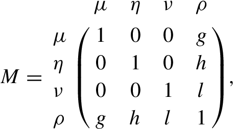
(13)
\[ S(A,B)=1-\frac{1}{n}{\sum \limits_{i=1}^{n}}\sqrt{\frac{1}{6}\big({I_{A}}({x_{i}})-{I_{B}}({x_{i}})\big)M{\big({I_{A}}({x_{i}})-{I_{B}}({x_{i}})\big)^{\mathrm{T}}}}.\]
$g,h,l\in [0,1]$, $g+h+l=1$. M is called a relationship matrix.
In this relationship matrix, we know that the relation value between positive membership and positive membership is 1. Similarly, the relation value between neutral memberships, negative memberships, refusal memberships are 1. Since the three component functions of picture fuzzy set are independent of each other, the relation value among positive membership, neutral membership and negative membership are 0. We assume that the values of the relationship between the refusal membership and positive membership, neutral membership, negative membership are g, h, l, respectively. It’s clear that g, h, l are not greater than one, and they add up to one.
Proof.
Let $A=\{\langle {\mu _{A}}({x_{i}}),{\eta _{A}}({x_{i}}),{\nu _{A}}({x_{i}})\rangle \mid {x_{i}}\in X\}$ and $B=\{\langle {\mu _{B}}({x_{i}}),{\eta _{B}}({x_{i}}),{\nu _{B}}({x_{i}})\rangle \mid {x_{i}}\in X\}$ be two picture fuzzy sets on X.
Taking a close explanation of the similarity measure $S(A,B)$:
\[\begin{aligned}{}& \big({I_{A}}({x_{i}})-{I_{B}}({x_{i}})\big)M{\big({I_{A}}({x_{i}})-{I_{B}}({x_{i}})\big)^{\mathrm{T}}}\\ {} & \hspace{1em}={\left(\begin{array}{c}{\mu _{A}}({x_{i}})-{\mu _{B}}({x_{i}})\\ {} {\eta _{A}}({x_{i}})-{\eta _{B}}({x_{i}})\\ {} {\nu _{A}}({x_{i}})-{\nu _{B}}({x_{i}})\\ {} {\rho _{A}}({x_{i}})-{\rho _{B}}({x_{i}})\end{array}\right)^{\mathrm{T}}}\left(\begin{array}{c@{\hskip4.0pt}c@{\hskip4.0pt}c@{\hskip4.0pt}c}1\hspace{1em}& 0\hspace{1em}& 0\hspace{1em}& g\\ {} 0\hspace{1em}& 1\hspace{1em}& 0\hspace{1em}& h\\ {} 0\hspace{1em}& 0\hspace{1em}& 1\hspace{1em}& l\\ {} g\hspace{1em}& h\hspace{1em}& l\hspace{1em}& 1\end{array}\right)\left(\begin{array}{c}{\mu _{A}}({x_{i}})-{\mu _{B}}({x_{i}})\\ {} {\eta _{A}}({x_{i}})-{\eta _{B}}({x_{i}})\\ {} {\nu _{A}}({x_{i}})-{\nu _{B}}({x_{i}})\\ {} {\rho _{A}}({x_{i}})-{\rho _{B}}({x_{i}})\end{array}\right)\\ {} & \hspace{1em}=(2-2g){\big({\mu _{A}}({x_{i}})-{\mu _{B}}({x_{i}})\big)^{2}}+(2-2h){\big({\eta _{A}}({x_{i}})-{\eta _{B}}({x_{i}})\big)^{2}}\\ {} & \hspace{2em}+(2-2l){\big({\nu _{A}}({x_{i}})-{\nu _{B}}({x_{i}})\big)^{2}}+(2-2g-2h)\big({\mu _{A}}({x_{i}})-{\mu _{B}}({x_{i}})\big)\\ {} & \hspace{2em}\times \big({\eta _{A}}({x_{i}})-{\eta _{B}}({x_{i}})\big)+(2-2g-2l)\big({\mu _{A}}({x_{i}})-{\mu _{B}}({x_{i}})\big)\big({\nu _{A}}({x_{i}})\\ {} & \hspace{2em}-{\nu _{B}}({x_{i}})\big)+(2-2h-2l)\big({\eta _{A}}({x_{i}})-{\eta _{B}}({x_{i}})\big)\big({\nu _{A}}({x_{i}})-{\nu _{B}}({x_{i}})\big).\end{aligned}\]
\[\begin{aligned}{}S(A,B)& =1-\frac{1}{n}{\sum \limits_{i=1}^{n}}\bigg\{\frac{1}{3}\big[(1-g){\big({\mu _{A}}({x_{i}})-{\mu _{B}}({x_{i}})\big)^{2}}\\ {} & \hspace{1em}+(1-h){\big({\eta _{A}}({x_{i}})-{\eta _{B}}({x_{i}})\big)^{2}}+(1-l){\big({\nu _{A}}({x_{i}})-{\nu _{B}}({x_{i}})\big)^{2}}\\ {} & \hspace{1em}+(1-g-h)\big({\mu _{A}}({x_{i}})-{\mu _{B}}({x_{i}})\big)\big({\eta _{A}}({x_{i}})-{\eta _{B}}({x_{i}})\big)\\ {} & \hspace{1em}+(1-g-l)\big({\mu _{A}}({x_{i}})-{\mu _{B}}({x_{i}})\big)\big({\nu _{A}}({x_{i}})-{\nu _{B}}({x_{i}})\big)\\ {} & \hspace{1em}+(1-h-l)\big({\eta _{A}}({x_{i}})-{\eta _{B}}({x_{i}})\big)\big({\nu _{A}}({x_{i}})-{\nu _{B}}({x_{i}})\big)\big]\bigg\}{^{\frac{1}{2}}}.\end{aligned}\]
(S1) For $A=\{\langle {\mu _{A}}({x_{i}}),{\eta _{A}}({x_{i}}),{\nu _{A}}({x_{i}})\rangle \mid {x_{i}}\in X\}$, $B=\{\langle {\mu _{B}}({x_{i}}),{\eta _{B}}({x_{i}}),{\nu _{B}}({x_{i}})\rangle \mid {x_{i}}\in X\}$, we have $-1\leqslant {\mu _{A}}({x_{i}})-{\mu _{B}}({x_{i}})\leqslant 1$, $-1\leqslant {\eta _{A}}({x_{i}})-{\eta _{B}}({x_{i}})\leqslant 1$ and $-1\leqslant {\nu _{A}}({x_{i}})-{\nu _{A}}({x_{i}})\leqslant 1$. Hence,
\[\begin{aligned}{}& {\big({\mu _{A}}({x_{i}})-{\mu _{B}}({x_{i}})\big)^{2}}\in [0,1],\hspace{1em}{\big({\eta _{A}}({x_{i}})-{\eta _{B}}({x_{i}})\big)^{2}}\in [0,1],\\ {} & {\big({\nu _{A}}({x_{i}})-{\nu _{B}}({x_{i}})\big)^{2}}\in [0,1],\hspace{1em}\big({\mu _{A}}({x_{i}})-{\mu _{B}}({x_{i}})\big)\big({\eta _{A}}({x_{i}})-{\eta _{B}}({x_{i}})\big)\in [-1,1],\\ {} & \big({\mu _{A}}({x_{i}})-{\mu _{B}}({x_{i}})\big)\big({\nu _{A}}({x_{i}})-{\nu _{B}}({x_{i}})\big)\in [-1,1],\\ {} & \big({\eta _{A}}({x_{i}})-{\eta _{B}}({x_{i}})\big)\big({\nu _{A}}({x_{i}})-{\nu _{B}}({x_{i}})\big)\in [-1,1],\\ {} & 1-g,1-h,1-l,1-g-h,1-g-l,1-h-l\in [0,1].\end{aligned}\]
\[\begin{aligned}{}& 1-\frac{1}{n}{\sum \limits_{i=1}^{n}}\bigg\{\frac{1}{3}\big[(1-g){\big({\mu _{A}}({x_{i}})-{\mu _{B}}({x_{i}})\big)^{2}}+(1-h){\big({\eta _{A}}({x_{i}})-{\eta _{B}}({x_{i}})\big)^{2}}\\ {} & \hspace{2em}+(1-l){\big({\nu _{A}}({x_{i}})-{\nu _{B}}({x_{i}})\big)^{2}}+(1-g-h)\big({\mu _{A}}({x_{i}})-{\mu _{B}}({x_{i}})\big)\\ {} & \hspace{2em}\times \big({\eta _{A}}({x_{i}})-{\eta _{B}}({x_{i}})\big)+(1-g-l)\big({\mu _{A}}({x_{i}})-{\mu _{B}}({x_{i}})\big)\big({\nu _{A}}({x_{i}})-{\nu _{B}}({x_{i}})\big)\\ {} & \hspace{2em}+(1-h-l)\big({\eta _{A}}({x_{i}})-{\eta _{B}}({x_{i}})\big)\big({\nu _{A}}({x_{i}})-{\nu _{B}}({x_{i}})\big)\big]\bigg\}{^{\frac{1}{2}}}\\ {} & \hspace{1em}\geqslant 1-\bigg\{\frac{1}{3}\big[(1-g)+(1-h)+(1-l)+(1-g-h)+(1-g-l)\\ {} & \hspace{2em}+(1-h-l)\big]\bigg\}{^{\frac{1}{2}}}=0.\end{aligned}\]
Besides,
\[\begin{aligned}{}& 1-\frac{1}{n}{\sum \limits_{i=1}^{n}}\bigg\{\frac{1}{3}\big[(1-g){\big({\mu _{A}}({x_{i}})-{\mu _{B}}({x_{i}})\big)^{2}}+(1-h){\big({\eta _{A}}({x_{i}})-{\eta _{B}}({x_{i}})\big)^{2}}\\ {} & \hspace{1em}+(1-l){\big({\nu _{A}}({x_{i}})-{\nu _{B}}({x_{i}})\big)^{2}}+(1-g-h)\big({\mu _{A}}({x_{i}})-{\mu _{B}}({x_{i}})\big)\\ {} & \hspace{1em}\times \big({\eta _{A}}({x_{i}})-{\eta _{B}}({x_{i}})\big)+(1-g-l)\big({\mu _{A}}({x_{i}})-{\mu _{B}}({x_{i}})\big)\big({\nu _{A}}({x_{i}})-{\nu _{B}}({x_{i}})\big)\\ {} & \hspace{1em}+(1-h-l)\big({\eta _{A}}({x_{i}})-{\eta _{B}}({x_{i}})\big)\big({\nu _{A}}({x_{i}})-{\nu _{B}}({x_{i}})\big)\big]\bigg\}{^{\frac{1}{2}}}\leqslant 1.\end{aligned}\]
Thus, we can get
\[\begin{aligned}{}0& \leqslant 1-\frac{1}{n}{\sum \limits_{i=1}^{n}}\bigg\{\frac{1}{3}\big[(1-g){\big({\mu _{A}}({x_{i}})-{\mu _{B}}({x_{i}})\big)^{2}}+(1-h){\big({\eta _{A}}({x_{i}})-{\eta _{B}}({x_{i}})\big)^{2}}\\ {} & \hspace{1em}+(1-l){\big({\nu _{A}}({x_{i}})-{\nu _{B}}({x_{i}})\big)^{2}}+(1-g-h)\big({\mu _{A}}({x_{i}})-{\mu _{B}}({x_{i}})\big)\\ {} & \hspace{1em}\times \big({\eta _{A}}({x_{i}})-{\eta _{B}}({x_{i}})\big)+(1-g-l)\big({\mu _{A}}({x_{i}})-{\mu _{B}}({x_{i}})\big)\big({\nu _{A}}({x_{i}})-{\nu _{B}}({x_{i}})\big)\\ {} & \hspace{1em}+(1-h-l)\big({\eta _{A}}({x_{i}})-{\eta _{B}}({x_{i}})\big)\big({\nu _{A}}({x_{i}})-{\nu _{B}}({x_{i}})\big)\big]\bigg\}{^{\frac{1}{2}}}\leqslant 1.\end{aligned}\]
From the above analysis, we get $0\leqslant S(A,B)\leqslant 1$.(S2) Obviously, $S(A,B)=S(B,A)$.
(S3)
\[\begin{aligned}{}& S(A,B)=1\\ {} & \hspace{1em}\Leftrightarrow \bigg\{\frac{1}{3}\big[(1-g){\big({\mu _{A}}({x_{i}})-{\mu _{B}}({x_{i}})\big)^{2}}+(1-h){\big({\eta _{A}}({x_{i}})-{\eta _{B}}({x_{i}})\big)^{2}}+(1-l)\\ {} & \hspace{2em}\times {\big({\nu _{A}}({x_{i}})-{\nu _{B}}({x_{i}})\big)^{2}}+(1-g-h)\big({\mu _{A}}({x_{i}})-{\mu _{B}}({x_{i}})\big)\big({\eta _{A}}({x_{i}})-{\eta _{B}}({x_{i}})\big)\\ {} & \hspace{2em}+(1-g-l)\big({\mu _{A}}({x_{i}})-{\mu _{B}}({x_{i}})\big)\big({\nu _{A}}({x_{i}})-{\nu _{B}}({x_{i}})\big)+(1-h-l)\\ {} & \hspace{2em}\times \big({\eta _{A}}({x_{i}})-{\eta _{B}}({x_{i}})\big)\big({\nu _{A}}({x_{i}})-{\nu _{B}}({x_{i}})\big)\big]\bigg\}{^{\frac{1}{2}}}=0\\ {} & \hspace{1em}\Leftrightarrow {\mu _{A}}({x_{i}})={\mu _{B}}({x_{i}}),{\eta _{A}}({x_{i}})={\eta _{B}}({x_{i}}),{\nu _{A}}({x_{i}})={\nu _{B}}({x_{i}}).\end{aligned}\]
Then from the above analysis, we get $S(A,B)=1$ if and only if $A=B$.(S4) Let $A=\{\langle {\mu _{A}}({x_{i}}),{\eta _{A}}({x_{i}}),{\nu _{A}}({x_{i}})\rangle \mid {x_{i}}\in X\}$, $B=\{\langle {\mu _{B}}({x_{i}}),{\eta _{B}}({x_{i}}),{\nu _{B}}({x_{i}})\rangle \mid {x_{i}}\in X\}$ and $C=\{\langle {\mu _{C}}({x_{i}})$, ${\eta _{C}}({x_{i}}),{\nu _{C}}({x_{i}})\rangle \mid {x_{i}}\in X\}$ be three PFSs that satisfy the relation $A\subseteq B\subseteq C$, we have:
\[\begin{aligned}{}S(B,C)& =1-\frac{1}{n}{\sum \limits_{i=1}^{n}}\bigg\{\frac{1}{3}\big[(1-g){\big({\mu _{B}}({x_{i}})-{\mu _{C}}({x_{i}})\big)^{2}}+(1-h){\big({\eta _{B}}({x_{i}})-{\eta _{C}}({x_{i}})\big)^{2}}\\ {} & \hspace{1em}+(1-l){\big({\nu _{B}}({x_{i}})-{\nu _{C}}({x_{i}})\big)^{2}}+(1-g-h)\big({\mu _{B}}({x_{i}})-{\mu _{C}}({x_{i}})\big)\\ {} & \hspace{1em}\times \big({\eta _{B}}({x_{i}})-{\eta _{C}}({x_{i}})\big)+(1-g-l)\big({\mu _{B}}({x_{i}})-{\mu _{C}}({x_{i}})\big)\big({\nu _{B}}({x_{i}})-{\nu _{C}}({x_{i}})\big)\\ {} & \hspace{1em}+(1-h-l)\big({\eta _{B}}({x_{i}})-{\eta _{C}}({x_{i}})\big)\big({\nu _{B}}({x_{i}})-{\nu _{C}}({x_{i}})\big)\big]\bigg\}{^{\frac{1}{2}}},\\ {} S(A,C)& =1-\frac{1}{n}{\sum \limits_{i=1}^{n}}\bigg\{\frac{1}{3}\big[(1-g){\big({\mu _{A}}({x_{i}})-{\mu _{C}}({x_{i}})\big)^{2}}+(1-h){\big({\eta _{A}}({x_{i}})-{\eta _{C}}({x_{i}})\big)^{2}}\\ {} & \hspace{1em}+(1-l){\big({\nu _{A}}({x_{i}})-{\nu _{C}}({x_{i}})\big)^{2}}+(1-g-h)\big({\mu _{A}}({x_{i}})-{\mu _{C}}({x_{i}})\big)\\ {} & \hspace{1em}\times \big({\eta _{A}}({x_{i}})-{\eta _{C}}({x_{i}})\big)+(1-g-l)\big({\mu _{A}}({x_{i}})-{\mu _{C}}({x_{i}})\big)\big({\nu _{A}}({x_{i}})-{\nu _{C}}({x_{i}})\big)\\ {} & \hspace{1em}+(1-h-l)\big({\eta _{A}}({x_{i}})-{\eta _{C}}({x_{i}})\big)\big({\nu _{A}}({x_{i}})-{\nu _{C}}({x_{i}})\big)\big]\bigg\}{^{\frac{1}{2}}},\\ {} S(A,B)& =1-\frac{1}{n}{\sum \limits_{i=1}^{n}}\bigg\{\frac{1}{3}\big[(1-g){\big({\mu _{A}}({x_{i}})-{\mu _{B}}({x_{i}})\big)^{2}}+(1-h){\big({\eta _{A}}({x_{i}})-{\eta _{B}}({x_{i}})\big)^{2}}\\ {} & \hspace{1em}+(1-l){\big({\nu _{A}}({x_{i}})-{\nu _{B}}({x_{i}})\big)^{2}}+(1-g-h)\big({\mu _{A}}({x_{i}})-{\mu _{B}}({x_{i}})\big)\\ {} & \hspace{1em}\times \big({\eta _{A}}({x_{i}})-{\eta _{B}}({x_{i}})\big)+(1-g-l)\big({\mu _{A}}({x_{i}})-{\mu _{B}}({x_{i}})\big)\big({\nu _{A}}({x_{i}})-{\nu _{B}}({x_{i}})\big)\\ {} & \hspace{1em}+(1-h-l)\big({\eta _{A}}({x_{i}})-{\eta _{B}}({x_{i}})\big)\big({\nu _{A}}({x_{i}})-{\nu _{B}}({x_{i}})\big)\big]\bigg\}{^{\frac{1}{2}}}.\end{aligned}\]
For $a,b,c,\in [0,1]$, $a+b+c\leqslant 1$, $x,y,z\in [0,1]$, $x+y+z\in [0,1]$. $1-g,1-h,1-l,1-g-h,1-g-l,1-h-l\in [0,1]$, we define a function f as:
\[\begin{aligned}{}f(x,y,z)& =\frac{1}{3}\big[(1-g){(x-a)^{2}}+(1-h){(y-b)^{2}}+(1-l){(z-c)^{2}}\\ {} & \hspace{1em}+(1-g-h)(x-a)(y-b)+(1-g-l)(x-a)(z-c)\\ {} & \hspace{1em}+(1-h-l)(y-b)(z-c)\big].\end{aligned}\]
We have
\[\begin{aligned}{}& \frac{\partial f}{\partial x}=\frac{1}{3}\big[2(1-g)(x-a)+(1-g-h)(y-b)+(1-g-l)(z-c)\big],\\ {} & \frac{\partial f}{\partial x}{\bigg|_{\genfrac{}{}{0pt}{}{y=b}{z=c}}}=\frac{1}{3}(1-g)(x-a),\\ {} & \frac{\partial f}{\partial y}=\frac{1}{3}\big[2(1-h)(y-b)+(1-g-h)(x-a)+(1-h-l)(z-c)\big],\\ {} & \frac{\partial f}{\partial y}{\bigg|_{\genfrac{}{}{0pt}{}{x=a}{z=c}}}=\frac{1}{3}(1-h)(y-b)\end{aligned}\]
and
\[\begin{aligned}{}& \frac{\partial f}{\partial z}=\frac{1}{3}\big[2(1-l)(z-c)+(1-g-l)(x-a)+(1-h-l)(y-b)\big],\\ {} & \frac{\partial f}{\partial z}{\bigg|_{\genfrac{}{}{0pt}{}{x=a}{y=b}}}=\frac{1}{3}(1-l)(z-c).\end{aligned}\]
Therefore, $\frac{\partial f}{\partial x}\leqslant 0$, for $0\leqslant x\leqslant a$. It means that f is a decreasing function of x, when $y=b$, $z=c$, $x\leqslant a$. Similarly, $\frac{\partial f}{\partial x}\geqslant 0$, for $a<x\leqslant 1$. It means that f is an increasing function of x, when $y=b$, $z=c$, $x>a$.In the same way, we can get $\frac{\partial f}{\partial y}\leqslant 0$ for $0\leqslant y\leqslant b$. It means that f is a decreasing function of y, when $x=a$, $z=c$, $y\leqslant b$. $\frac{\partial f}{\partial y}\geqslant 0$ for $b<y\leqslant 1$. It means that f is an increasing function of y, when $x=a$, $z=c$, $y>b$. $\frac{\partial f}{\partial z}\leqslant 0$ for $0\leqslant z\leqslant c$. It means that f is a decreasing function of z, when $x=a$, $y=b$, $z\leqslant c$. $\frac{\partial f}{\partial z}\geqslant 0$ for $c<z\leqslant 1$. It means that f is an increasing function of z, when $x=a$, $y=b$, $z>c$.
(1) Suppose that $A=\{\langle {\mu _{A}}({x_{i}}),{\eta _{A}}({x_{i}}),{\nu _{A}}({x_{i}})\rangle |{x_{i}}\in X\}$, $B=\{\langle {\mu _{B}}({x_{i}}),{\eta _{B}}({x_{i}}),{\nu _{B}}({x_{i}})\rangle |{x_{i}}\in X\}$ and $C=\{\langle {\mu _{C}}({x_{i}}),{\eta _{C}}({x_{i}}),{\nu _{C}}({x_{i}})|{x_{i}}\in X\rangle \}$ satisfying
\[ \big({\mu _{A}}({x_{i}})<{\mu _{B}}({x_{i}})<{\mu _{C}}({x_{i}})\big)\wedge \big({\nu _{A}}({x_{i}})\geqslant {\nu _{B}}({x_{i}})\geqslant {\nu _{C}}({x_{i}})\big),\]
we can obtain:
\[\begin{aligned}{}f\big({\mu _{A}}({x_{i}}),{\mu _{A}}({x_{i}}),{\mu _{A}}({x_{i}})\big)& \leqslant f\big({\mu _{B}}({x_{i}}),{\eta _{B}}({x_{i}}),{\nu _{B}}({x_{i}})\big)\\ {} & \leqslant f\big({\mu _{C}}({x_{i}}),{\eta _{C}}({x_{i}}),{\nu _{C}}({x_{i}})\big),\end{aligned}\]
then:
\[\begin{aligned}{}& f\big({\mu _{B}}({x_{i}}),{\eta _{B}}({x_{i}}),{\nu _{B}}({x_{i}})\big)\leqslant f\big({\mu _{C}}({x_{i}}),{\eta _{C}}({x_{i}}),{\nu _{C}}({x_{i}})\big),\end{aligned}\]
i.e.
\[\begin{aligned}{}& \frac{1}{3}\big[(1-g){\big({\mu _{B}}({x_{i}})-{\mu _{A}}({x_{i}})\big)^{2}}+(1-h){\big({\eta _{B}}({x_{i}})-{\eta _{A}}({x_{i}})\big)^{2}}+(1-l)\\ {} & \hspace{2em}\times {\big({\nu _{B}}({x_{i}})-{\nu _{A}}({x_{i}})\big)^{2}}+(1-g-h)\big({\mu _{B}}({x_{i}})-{\mu _{A}}({x_{i}})\big)\big({\eta _{B}}({x_{i}})-{\eta _{A}}({x_{i}})\big)\\ {} & \hspace{2em}+(1-g-l)\big({\mu _{B}}({x_{i}})-{\mu _{A}}({x_{i}})\big)\big({\nu _{B}}({x_{i}})-{\nu _{A}}({x_{i}})\big)\\ {} & \hspace{2em}+(1-h-l)\big({\eta _{B}}({x_{i}})-{\eta _{A}}({x_{i}})\big)\big({\nu _{B}}({x_{i}})-{\nu _{A}}({x_{i}})\big)\big]\\ {} & \hspace{1em}\leqslant \frac{1}{3}\big[(1-g){\big({\mu _{C}}({x_{i}})-{\mu _{A}}({x_{i}})\big)^{2}}+(1-h){\big({\eta _{C}}({x_{i}})-{\eta _{A}}({x_{i}})\big)^{2}}+(1-l)\\ {} & \hspace{2em}\times {\big({\nu _{C}}({x_{i}})-{\nu _{A}}({x_{i}})\big)^{2}}+(1-g-h)\big({\mu _{C}}({x_{i}})-{\mu _{A}}({x_{i}})\big)\big({\eta _{C}}({x_{i}})-{\eta _{A}}({x_{i}})\big)\\ {} & \hspace{2em}+(1-g-l)\big({\mu _{C}}({x_{i}})-{\mu _{A}}({x_{i}})\big)\big({\nu _{C}}({x_{i}})-{\nu _{A}}({x_{i}})\big)\\ {} & \hspace{2em}+(1-h-l)\big({\eta _{C}}({x_{i}})-{\eta _{A}}({x_{i}})\big)\big({\nu _{C}}({x_{i}})-{\nu _{A}}({x_{i}})\big)\big].\end{aligned}\]
Thus, we have:
\[\begin{aligned}{}& 1-\frac{1}{n}{\sum \limits_{i=1}^{n}}\bigg\{\frac{1}{3}\big[(1-g){\big({\mu _{A}}({x_{i}})-{\mu _{B}}({x_{i}})\big)^{2}}+(1-h){\big({\eta _{A}}({x_{i}})-{\eta _{B}}({x_{i}})\big)^{2}}\\ {} & \hspace{2em}+(1-l){\big({\nu _{A}}({x_{i}})-{\nu _{B}}({x_{i}})\big)^{2}}+(1-g-h)\big({\mu _{A}}({x_{i}})-{\mu _{B}}({x_{i}})\big)\\ {} & \hspace{2em}\times \big({\eta _{A}}({x_{i}})-{\eta _{B}}({x_{i}})\big)+(1-g-l)\big({\mu _{A}}({x_{i}})-{\mu _{B}}({x_{i}})\big)\big({\nu _{A}}({x_{i}})-{\nu _{B}}({x_{i}})\big)\\ {} & \hspace{2em}+(1-h-l)\big({\eta _{A}}({x_{i}})-{\eta _{B}}({x_{i}})\big)\big({\nu _{A}}({x_{i}})-{\nu _{B}}({x_{i}})\big)\big]\bigg\}{^{\frac{1}{2}}}\\ {} & \hspace{1em}\geqslant 1-\frac{1}{n}{\sum \limits_{i=1}^{n}}\bigg\{\frac{1}{3}\big[(1-g){\big({\mu _{A}}({x_{i}})-{\mu _{C}}({x_{i}})\big)^{2}}+(1-h){\big({\eta _{A}}({x_{i}})-{\eta _{C}}({x_{i}})\big)^{2}}\\ {} & \hspace{2em}+(1-l){\big({\nu _{A}}({x_{i}})-{\nu _{C}}({x_{i}})\big)^{2}}+(1-g-h)\big({\mu _{A}}({x_{i}})-{\mu _{C}}({x_{i}})\big)\\ {} & \hspace{2em}\times \big({\eta _{A}}({x_{i}})-{\eta _{C}}({x_{i}})\big)+(1-g-l)\big({\mu _{A}}({x_{i}})-{\mu _{C}}({x_{i}})\big)\big({\nu _{A}}({x_{i}})-{\nu _{C}}({x_{i}})\big)\\ {} & \hspace{2em}+(1-h-l)\big({\eta _{A}}({x_{i}})-{\eta _{C}}({x_{i}})\big)\big({\nu _{A}}({x_{i}})-{\nu _{C}}({x_{i}})\big)\big]\bigg\}{^{\frac{1}{2}}}.\end{aligned}\]
$S(A,B)\geqslant S(A,C)$ is founded. Similarly, if we suppose $a={\mu _{C}}$, $b={\eta _{C}}$, $c={\nu _{C}}$, then we have $S(B,C)\geqslant S(A,C)$.(2) Suppose that $A=\{\langle {\mu _{A}}({x_{i}}),{\eta _{A}}({x_{i}}),{\nu _{A}}({x_{i}})\rangle \mid {x_{i}}\in X\}$, $B=\{\langle {\mu _{B}}({x_{i}}),{\eta _{B}}({x_{i}}),{\nu _{B}}({x_{i}})\rangle \mid {x_{i}}\in X\}$ and $C=\{\langle {\mu _{C}}({x_{i}}),{\eta _{C}}({x_{i}}),{\nu _{C}}({x_{i}})\rangle \mid {x_{i}}\in X\}$ satisfying
\[ \big({\mu _{A}}({x_{i}})={\mu _{B}}({x_{i}})={\mu _{C}}({x_{i}})\big)\wedge \big({\nu _{A}}({x_{i}})>{\nu _{B}}({x_{i}})>{\nu _{C}}({x_{i}})\big),\]
we can obtain
\[\begin{aligned}{}f\big({\mu _{A}}({x_{i}}),{\mu _{B}}({x_{i}}),{\mu _{C}}({x_{i}})\big)& \leqslant f\big({\mu _{B}}({x_{i}}),{\eta _{B}}({x_{i}}),{\nu _{B}}({x_{i}})\big)\\ {} & \leqslant f\big({\mu _{C}}({x_{i}}),{\eta _{C}}({x_{i}}),{\nu _{C}}({x_{i}})\big).\end{aligned}\]
Thus, we have:
\[\begin{aligned}{}& 1-\frac{1}{n}{\sum \limits_{i=1}^{n}}\bigg\{\frac{1}{3}\big[(1-g){\big({\mu _{A}}({x_{i}})-{\mu _{B}}({x_{i}})\big)^{2}}+(1-h){\big({\eta _{A}}({x_{i}})-{\eta _{B}}({x_{i}})\big)^{2}}\\ {} & \hspace{2em}+(1-l){\big({\nu _{A}}({x_{i}})-{\nu _{B}}({x_{i}})\big)^{2}}+(1-g-h)\big({\mu _{A}}({x_{i}})-{\mu _{B}}({x_{i}})\big)\\ {} & \hspace{2em}\times \big({\eta _{A}}({x_{i}})-{\eta _{B}}({x_{i}})\big)+(1-g-l)\big({\mu _{A}}({x_{i}})-{\mu _{B}}({x_{i}})\big)\big({\nu _{A}}({x_{i}})-{\nu _{B}}({x_{i}})\big)\\ {} & \hspace{2em}+(1-h-l)\big({\eta _{A}}({x_{i}})-{\eta _{B}}({x_{i}})\big)\big({\nu _{A}}({x_{i}})-{\nu _{B}}({x_{i}})\big)\big]\bigg\}{^{\frac{1}{2}}}\\ {} & \hspace{1em}\geqslant 1-\frac{1}{n}{\sum \limits_{i=1}^{n}}\bigg\{\frac{1}{3}\big[(1-g){\big({\mu _{A}}({x_{i}})-{\mu _{C}}({x_{i}})\big)^{2}}+(1-h){\big({\eta _{A}}({x_{i}})-{\eta _{C}}({x_{i}})\big)^{2}}\\ {} & \hspace{2em}+(1-l){\big({\nu _{A}}({x_{i}})-{\nu _{C}}({x_{i}})\big)^{2}}+(1-g-h)\big({\mu _{A}}({x_{i}})-{\mu _{C}}({x_{i}})\big)\\ {} & \hspace{2em}\times \big({\eta _{A}}({x_{i}})-{\eta _{C}}({x_{i}})\big)+(1-g-l)\big({\mu _{A}}({x_{i}})-{\mu _{C}}({x_{i}})\big)\big({\nu _{A}}({x_{i}})-{\nu _{C}}({x_{i}})\big)\\ {} & \hspace{2em}+(1-h-l)\big({\eta _{A}}({x_{i}})-{\eta _{C}}({x_{i}})\big)\big({\nu _{A}}({x_{i}})-{\nu _{C}}({x_{i}})\big)\big]\bigg\}{^{\frac{1}{2}}}.\end{aligned}\]
$S(A,B)\geqslant S(A,C)$ is founded. Similarly, if we suppose $a={\mu _{C}}$, $b={\eta _{C}}$, $c={\nu _{C}}$, then we have $S(B,C)\geqslant S(A,C)$.(3) Suppose that $A=\{\langle {\mu _{A}}({x_{i}}),{\eta _{A}}({x_{i}}),{\nu _{A}}({x_{i}})\rangle \mid {x_{i}}\in X\}$, $B=\{\langle {\mu _{B}}({x_{i}}),{\eta _{B}}({x_{i}}),{\nu _{B}}({x_{i}})\rangle \mid {x_{i}}\in X\}$ and $C=\{\langle {\mu _{C}}({x_{i}}),{\eta _{C}}({x_{i}}),{\nu _{C}}({x_{i}})\rangle \mid {x_{i}}\in X\}$ satisfying
\[\begin{aligned}{}\big({\mu _{A}}({x_{i}})={\mu _{B}}({x_{i}})={\mu _{C}}({x_{i}})\big)& \wedge \big({\nu _{A}}({x_{i}})={\nu _{B}}({x_{i}})={\nu _{C}}({x_{i}})\big)\\ {} & \wedge \big({\eta _{A}}({x_{i}})\leqslant {\eta _{B}}({x_{i}})\leqslant {\eta _{C}}({x_{i}})\big),\end{aligned}\]
we can obtain
\[\begin{aligned}{}f\big({\mu _{A}}({x_{i}}),{\mu _{B}}({x_{i}}),{\mu _{C}}({x_{i}})\big)& \leqslant f\big({\mu _{B}}({x_{i}}),{\eta _{B}}({x_{i}}),{\nu _{B}}({x_{i}})\big)\\ {} & \leqslant f\big({\mu _{C}}({x_{i}}),{\eta _{C}}({x_{i}}),{\nu _{C}}({x_{i}})\big).\end{aligned}\]
Thus we have
\[\begin{aligned}{}& 1-\frac{1}{n}{\sum \limits_{i=1}^{n}}\bigg\{\frac{1}{3}\big[(1-g){\big({\mu _{A}}({x_{i}})-{\mu _{B}}({x_{i}})\big)^{2}}+(1-h){\big({\eta _{A}}({x_{i}})-{\eta _{B}}({x_{i}})\big)^{2}}\\ {} & \hspace{2em}+(1-l){\big({\nu _{A}}({x_{i}})-{\nu _{B}}({x_{i}})\big)^{2}}+(1-g-h)\big({\mu _{A}}({x_{i}})-{\mu _{B}}({x_{i}})\big)\\ {} & \hspace{2em}\times \big({\eta _{A}}({x_{i}})-{\eta _{B}}({x_{i}})\big)+(1-g-l)\big({\mu _{A}}({x_{i}})-{\mu _{B}}({x_{i}})\big)\big({\nu _{A}}({x_{i}})-{\nu _{B}}({x_{i}})\big)\\ {} & \hspace{2em}+(1-h-l)\big({\eta _{A}}({x_{i}})-{\eta _{B}}({x_{i}})\big)\big({\nu _{A}}({x_{i}})-{\nu _{B}}({x_{i}})\big)\big]\bigg\}{^{\frac{1}{2}}}\\ {} & \hspace{1em}\geqslant 1-\frac{1}{n}{\sum \limits_{i=1}^{n}}\bigg\{\frac{1}{3}\big[(1-g){\big({\mu _{A}}({x_{i}})-{\mu _{C}}({x_{i}})\big)^{2}}+(1-h){\big({\eta _{A}}({x_{i}})-{\eta _{C}}({x_{i}})\big)^{2}}\\ {} & \hspace{2em}+(1-l){\big({\nu _{A}}({x_{i}})-{\nu _{C}}({x_{i}})\big)^{2}}+(1-g-h)\big({\mu _{A}}({x_{i}})-{\mu _{C}}({x_{i}})\big)\\ {} & \hspace{2em}\times \big({\eta _{A}}({x_{i}})-{\eta _{C}}({x_{i}})\big)+(1-g-l)\big({\mu _{A}}({x_{i}})-{\mu _{C}}({x_{i}})\big)\big({\nu _{A}}({x_{i}})-{\nu _{C}}({x_{i}})\big)\\ {} & \hspace{2em}+(1-h-l)\big({\eta _{A}}({x_{i}})-{\eta _{C}}({x_{i}})\big)\big({\nu _{A}}({x_{i}})-{\nu _{C}}({x_{i}})\big)\big]\bigg\}{^{\frac{1}{2}}}.\end{aligned}\]
$S(A,B)\geqslant S(A,C)$ is founded. Similarly, if we suppose $a={\mu _{C}}$, $b={\eta _{C}}$, $c={\nu _{C}}$, then we can get $S(B,C)\geqslant S(A,C)$.Furthermore, picture fuzzy sets $A=\{\langle {\mu _{A}}({x_{i}}),{\eta _{A}}({x_{i}}),{\nu _{A}}({x_{i}})\rangle \mid {x_{i}}\in X\}$, $B=\{\langle {\mu _{B}}({x_{i}}),{\eta _{B}}({x_{i}}),{\nu _{B}}({x_{i}})\rangle \mid {x_{i}}\in X\}$ and $C=\{\langle {\mu _{C}}({x_{i}}),{\eta _{C}}({x_{i}}),{\nu _{C}}({x_{i}})\rangle \mid {x_{i}}\in X\}$, $A\subseteq B\subseteq C$ also satisfying
(4) $({\mu _{A}}({x_{i}})<{\mu _{B}}({x_{i}})={\mu _{C}}({x_{i}}))\wedge ({\nu _{A}}({x_{i}})\geqslant {\nu _{B}}({x_{i}})>{\nu _{C}}({x_{i}}))$.
(5) $({\mu _{A}}({x_{i}})<{\mu _{B}}({x_{i}})={\mu _{C}}({x_{i}}))\wedge ({\nu _{A}}({x_{i}})\geqslant {\nu _{B}}({x_{i}})={\nu _{C}}({x_{i}}))\wedge ({\eta _{B}}({x_{i}})\leqslant {\eta _{C}}({x_{i}}))$.
(6) $({\mu _{A}}({x_{i}})={\mu _{B}}({x_{i}})<{\mu _{C}}({x_{i}}))\wedge ({\nu _{A}}({x_{i}})>{\nu _{B}}({x_{i}})\geqslant {\nu _{C}}({x_{i}}))$.
(7) $({\mu _{A}}({x_{i}})={\mu _{B}}({x_{i}})={\mu _{C}}({x_{i}}))\wedge ({\nu _{A}}({x_{i}})>{\nu _{B}}({x_{i}})={\nu _{C}}({x_{i}}))\wedge ({\eta _{B}}({x_{i}})\leqslant {\eta _{C}}({x_{i}}))$.
(8) $({\mu _{A}}({x_{i}})={\mu _{B}}({x_{i}})<{\mu _{C}}({x_{i}}))\wedge ({\nu _{A}}({x_{i}})={\nu _{B}}({x_{i}})\geqslant {\nu _{C}}({x_{i}}))\wedge ({\eta _{A}}({x_{i}})\leqslant {\eta _{B}}({x_{i}}))$.
(9) $({\mu _{A}}({x_{i}})={\mu _{B}}({x_{i}})={\mu _{C}}({x_{i}}))\wedge ({\nu _{B}}({x_{i}})>{\nu _{C}}({x_{i}}))\wedge ({\eta _{A}}({x_{i}})\leqslant {\eta _{B}}({x_{i}}))$.
Similarly, these cases can be proved.
Remark 3.1.
Let $A=\{\langle {\mu _{A}}({x_{i}}),{\eta _{A}}({x_{i}}),{\nu _{A}}({x_{i}})\rangle \mid {x_{i}}\in X\}$ and $B=\{\langle {\mu _{B}}({x_{i}}),{\eta _{B}}({x_{i}}),{\nu _{B}}({x_{i}})\rangle \mid {x_{i}}\in X\}$ be two picture fuzzy sets on $X=\{{x_{1}},{x_{2}},\dots ,{x_{n}}\}$, then similarity measure between picture fuzzy sets A and B
where 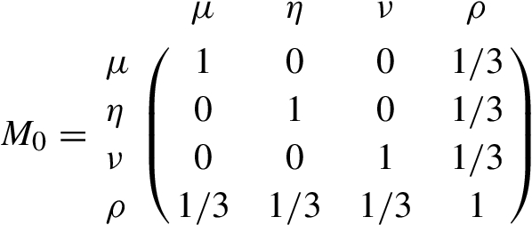 .
.
(14)
\[\begin{aligned}{}{S_{0}}(A,B)=& 1-\frac{1}{n}{\sum \limits_{i=1}^{n}}\sqrt{\frac{1}{6}\big({I_{A}}({x_{i}})-{I_{B}}({x_{i}})\big){M_{0}}{\big({I_{A}}({x_{i}})-{I_{B}}({x_{i}})\big)^{\mathrm{T}}}},\end{aligned}\]Remark 3.2.
If picture fuzzy sets A and B degenerate into intuitionistic fuzzy sets, the similarity measure
is a new similarity measure between intuitionistic fuzzy sets A and B, where ${I_{A}}({x_{i}})=[{\mu _{A}}({x_{i}}),{\nu _{A}}({x_{i}}),{\pi _{A}}({x_{i}})]$, ${I_{B}}({x_{i}})=[{\mu _{B}}({x_{i}}),{\nu _{B}}({x_{i}}),{\pi _{B}}({x_{i}})]$, 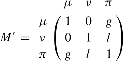 , and $g,l\in [0,1]$, $g+l=1$.
(15)
\[\begin{aligned}{}{S^{\prime }}(A,B)=& 1-\frac{1}{n}{\sum \limits_{i=1}^{n}}\sqrt{\frac{1}{2}\big({I_{A}}({x_{i}})-{I_{B}}({x_{i}})\big){M^{\prime }}{\big({I_{A}}({x_{i}})-{I_{B}}({x_{i}})\big)^{\mathrm{T}}}}\end{aligned}\]Theorem 3.2.
Let $A=\{\langle {\mu _{A}}({x_{i}}),{\eta _{A}}({x_{i}}),{\nu _{A}}({x_{i}})\rangle \mid {x_{i}}\in X\}$ and $B=\{\langle {\mu _{B}}({x_{i}}),{\eta _{B}}({x_{i}}),{\nu _{B}}({x_{i}})\rangle \mid {x_{i}}\in X\}$ be two picture fuzzy sets on $X=\{{x_{1}},{x_{2}},\dots ,{x_{n}}\}$. The mapping ${S_{w}}(A,B):\mathit{PFS}(X)\times \mathit{PFS}(X)\to [0,1]$ is defined as follows:
Then ${S_{w}}(A,B)$ is a similarity measure between A and B, where ${w_{i}}$ is the weight of ${x_{i}}$ on X, ${w_{i}}\in [0,1]$ and ${\textstyle\sum _{i=1}^{n}}{w_{i}}=1$.
(16)
\[\begin{aligned}{}& {S_{w}}(A,B)\\ {} & \hspace{1em}=1-{\sum \limits_{i=1}^{n}}{w_{i}}\bigg\{\frac{1}{3}\big[(1-g){\big({\mu _{A}}({x_{i}})-{\mu _{B}}({x_{i}})\big)^{2}}+(1-h){\big({\eta _{A}}({x_{i}})-{\eta _{B}}({x_{i}})\big)^{2}}\\ {} & \hspace{2em}+(1-l){\big({\nu _{A}}({x_{i}})-{\nu _{B}}({x_{i}})\big)^{2}}+(1-g-h)\big({\mu _{A}}({x_{i}})-{\mu _{B}}({x_{i}})\big)\\ {} & \hspace{2em}\times \big({\eta _{A}}({x_{i}})-{\eta _{B}}({x_{i}})\big)+(1-g-l)\big({\mu _{A}}({x_{i}})-{\mu _{B}}({x_{i}})\big)\\ {} & \hspace{2em}\times \big({\nu _{A}}({x_{i}})-{\nu _{B}}({x_{i}})\big)+(1-h-l)\big({\eta _{A}}({x_{i}})-{\eta _{B}}({x_{i}})\big)\big({\nu _{A}}({x_{i}})-{\nu _{B}}({x_{i}})\big)\big]\bigg\}{^{\frac{1}{2}}}.\end{aligned}\]4 Applications
In this section, a numerical example is constructed. Some of the existing similarity measures cannot produce rational results, while the proposed similarity measure can get a logical result. Then we apply the proposed similarity measure to multi-attribute decision making.
4.1 Numerical Comparisons
Example 4.1.
By comparing the first pairs of picture fuzzy sets $\{{A_{1}},{B_{1}}\}$ and $\{{A_{2}},{B_{2}}\}$, ${S_{{p_{1}}}}({A_{1}},{B_{1}})={S_{{p_{1}}}}({A_{2}},{B_{2}})$ when ${A_{1}}={A_{2}}$, ${B_{1}}\ne {B_{2}}$, we find that similarity measures ${S_{{p_{1}}}}$, ${S_{{p_{2}}}}$, ${S_{{p_{3}}}}$, ${S_{{p_{4}}}}$, ${S_{{g_{2}}}}$, ${S_{{g_{3}}}}$, ${S_{{g_{4}}}}$ have the same unreasonable results. Analogously, by comparing the other pairs of picture fuzzy sets $\{{A_{3}},{B_{3}}\}$, $\{{A_{4}},{B_{4}}\}$, we have irrational cases in ${S_{{p_{1}}}}$, ${S_{{p_{3}}}}$, ${S_{{p_{4}}}}$, ${S_{{g_{1}}}}$, ${S_{{g_{2}}}}$, ${S_{{g_{4}}}}$, ${S_{{w_{1}}}}$, ${S_{{w_{2}}}}$ as well. As can be seen from Table 1, there is no unreasonable result for the proposed similarity measure. It is more suitable to distinguish picture fuzzy sets.
4.2 Algorithm and Applications
4.2.1 Algorithm for Multi-Attribute Decision Making
Let $A=\{{A_{1}},{A_{1}},\dots ,{A_{n}}\}$ be a set of alternatives, $C=\{{C_{1}},{C_{2}},\dots ,{C_{m}}\}$ be a set of evaluation attributes. The weight vectors of different attributes are represented by ${w_{j}}=\{{w_{1}},{w_{2}},\dots ,{w_{m}}\}$, ${w_{j}}>0$, ${\textstyle\sum _{j=1}^{m}}{w_{j}}=1$. Suppose the picture fuzzy information is given by decision maker’s preference expressed as ${\delta _{ij}}=\langle {\mu _{ij}},{\eta _{ij}},{\nu _{ij}}\rangle $, $(i=1,2,\dots ,n$), ($j=1,2,\dots ,m$). The picture fuzzy decision matrix $R={({\delta _{ij}})_{n\times m}}$ is constructed according to the preference for the alternatives ${A_{i}}$ $(i=1,2,\dots ,n)$. The computational steps are explored as follows:
Step 1. Attributes may be divided into two types: cost attribute $(O)$ and benefit attribute $(E)$. We transform $R={({\delta _{ij}})_{n\times m}}$ into normalized picture fuzzy decision matrix $N={({\gamma _{ij}})_{n\times m}}$ according to the following equation:
Step 2. Let ${A^{+}}=\{{C_{1}^{+}},{C_{2}^{+}},\dots ,{C_{m}^{+}}\}$ be the ideal alternative. Each attribute value of the ideal alternative is expressed by maximum picture fuzzy number, then ${A^{+}}$ is shown as follows:
Step 4. Rank all alternatives ${A_{i}}$ $(i=1,2,\dots ,n)$ in a descending order in line with the value of the similarity. The best alternative is the one with the maximal similarity measure.
4.2.2 Applications for Multi-Attribute Decision Making
Example 4.2.
Joshi and Kumar (2018) consider an Indian multinational is planning its financial strategy in line with the group’s strategic objectives. After preliminary screening, four alternatives were obtained and determined as: ${A_{1}}$: to invest the “Southern Asian marketplace”, ${A_{2}}$: to invest the “Eastern Asian marketplace”, ${A_{3}}$: to invest the “Northern Asian marketplace”, ${A_{4}}$: to invest the “Local marketplace”. Evaluation attribute comes from four aspects: ${C_{1}}$: the risk analysis, ${C_{2}}$: the growth analysis, ${C_{3}}$: the sociopolitical influence, ${C_{4}}$: the environmental implication. The weight vector is $w={(0.2,0.3,0.1,0.4)^{\mathrm{T}}}$. Picture fuzzy decision matrix is constructed in Table 2.
Step 1. ${C_{2}}$ and ${C_{3}}$ are the benefit attributes while ${C_{1}}$ and ${C_{4}}$ are the cost attributes, we get the normalized picture fuzzy decision matrix in Table 3.
Table 2
Picture fuzzy decision matrix.
| ${C_{1}}$ | ${C_{2}}$ | ${C_{3}}$ | ${C_{4}}$ | |
| ${A_{1}}$ | $\langle 0.2,0.1,0.6\rangle $ | $\langle 0.5,0.3,0.1\rangle $ | $\langle 0.5,0.1,0.3\rangle $ | $\langle 0.4,0.3,0.2\rangle $ |
| ${A_{2}}$ | $\langle 0.1,0.4,0.4\rangle $ | $\langle 0.6,0.3,0.1\rangle $ | $\langle 0.2,0.1,0.7\rangle $ | $\langle 0.2,0.1,0.7\rangle $ |
| ${A_{3}}$ | $\langle 0.3,0.2,0.2\rangle $ | $\langle 0.6,0.2,0.1\rangle $ | $\langle 0.3,0.3,0.4\rangle $ | $\langle 0.3,0.3,0.4\rangle $ |
| ${A_{4}}$ | $\langle 0.3,0.1,0.6\rangle $ | $\langle 0.1,0.2,0.6\rangle $ | $\langle 0.2,0.3,0.2\rangle $ | $\langle 0.2,0.3,0.2\rangle $ |
Step 2. The ideal alternative is ${A^{+}}=\{{1_{{D^{\ast }}}},{1_{{D^{\ast }}}},{1_{{D^{\ast }}}},{1_{{D^{\ast }}}}\}$.
Table 3
Normalized picture fuzzy decision matrix.
| ${C_{1}}$ | ${C_{2}}$ | ${C_{3}}$ | ${C_{4}}$ | |
| ${A_{1}}$ | $\langle 0.6,0.1,0.2\rangle $ | $\langle 0.5,0.3,0.1\rangle $ | $\langle 0.5,0.1,0.3\rangle $ | $\langle 0.2,0.3,0.4\rangle $ |
| ${A_{2}}$ | $\langle 0.4,0.4,0.1\rangle $ | $\langle 0.6,0.3,0.1\rangle $ | $\langle 0.2,0.1,0.7\rangle $ | $\langle 0.7,0.1,0.2\rangle $ |
| ${A_{3}}$ | $\langle 0.2,0.2,0.3\rangle $ | $\langle 0.6,0.2,0.1\rangle $ | $\langle 0.3,0.3,0.4\rangle $ | $\langle 0.4,0.3,0.3\rangle $ |
| ${A_{4}}$ | $\langle 0.6,0.1,0.3\rangle $ | $\langle 0.1,0.2,0.6\rangle $ | $\langle 0.2,0.3,0.2\rangle $ | $\langle 0.2,0.3,0.2\rangle $ |
Step 3. We calculate the similarity measure $S({A_{i}},{A^{+}})$ $(i=1,2,3,4)$ by Theorem 3.2, where g, h, l were selected as $g=h=l=1/3$ and $g=1/6$, $h=1/2$, $l=1/3$. The results are shown in Table 4.
Step 4. The maximal similarity is the best one, the ranking results are shown in Table 5.
From the above results, it is clear that the best financial strategy is ${A_{2}}$. So we suggest the multinational to invest in Asian market. It can be seen from Table 5 that the different parameters may cause changes in the value of similarity measure, but does not affect the final decision. In Table 6, by comparing with the existing methods, it can be seen that our results are the same as the methods in literature (Garg, 2017; Joshi and Kumar, 2018).
Example 4.3.
Wei et al. (2018) consider an organization intends to select a promising emerging technology commercial enterprise. After their preliminary screening five enterprises are expressed as ${A_{1}}$, ${A_{2}}$, ${A_{3}}$, ${A_{4}}$, ${A_{5}}$. Evaluation attribute comes from four aspects: ${C_{1}}$: the technical progress, ${C_{2}}$: the potential market and market risk, ${C_{3}}$: the sociopolitical influence, ${C_{4}}$: the financial investment. The weight vector is $w={(0.2,0.1,0.3,0.4)^{\mathrm{T}}}$. Picture fuzzy decision matrix is constructed in Table 7.
Table 7
Normalized picture fuzzy decision matrix.
| ${C_{1}}$ | ${C_{2}}$ | ${C_{3}}$ | ${C_{4}}$ | |
| ${A_{1}}$ | $\langle 0.56,0.34,0.10\rangle $ | $\langle 0.90,0.07,0.03\rangle $ | $\langle 0.40,0.33,0.19\rangle $ | $\langle 0.09,0.79,0.03\rangle $ |
| ${A_{2}}$ | $\langle 0.70,0.10,0.09\rangle $ | $\langle 0.10,0.66,0.20\rangle $ | $\langle 0.06,0.81,0.12\rangle $ | $\langle 0.72,0.14,0.09\rangle $ |
| ${A_{3}}$ | $\langle 0.88,0.09,0.03\rangle $ | $\langle 0.08,0.10,0.06\rangle $ | $\langle 0.05,0.83,0.09\rangle $ | $\langle 0.65,0.25,0.07\rangle $ |
| ${A_{4}}$ | $\langle 0.80,0.07,0.04\rangle $ | $\langle 0.70,0.15,0.11\rangle $ | $\langle 0.03,0.88,0.05\rangle $ | $\langle 0.07,0.82,0.05\rangle $ |
| ${A_{5}}$ | $\langle 0.85,0.06,0.03\rangle $ | $\langle 0.64,0.07,0.22\rangle $ | $\langle 0.06,0.88,0.05\rangle $ | $\langle 0.13,0.77,0.09\rangle $ |
Step 1. ${C_{1}}$, ${C_{2}}$, ${C_{3}}$, ${C_{4}}$ are benefit attributes, the normalized decision matrix is picture fuzzy decision matrix.
Step 2. The ideal alternative is ${A^{+}}=\{{1_{{D^{\ast }}}},{1_{{D^{\ast }}}},{1_{{D^{\ast }}}},{1_{{D^{\ast }}}}\}$.
Step 3. We calculate the similarity measure $S({A_{i}},{A^{+}})(i=1,2,3,4)$ by Theorem 3.2, where g, h, l were selected as $g=h=l=1/3$ and $g=1/6$, $h=1/2$, $l=1/3$. The results are shown in Table 8.
Step 4. The maximal similarity is the best one, we get ranking results in Table 9.
From the above discussion, it is clear that the most promising enterprise is ${A_{3}}$. So we suggest the organization to pick the enterprise ${A_{3}}$. In Table 8, we can also see that the different values of parameters may lead to the changes in the value of similarity measure, but does not affect the final decision. From Table 10, by comparing with other methods, it can be seen that our results are consistent with the methods in Wei (2018, 2017a).
Example 4.4.
Table 11
Normalized picture fuzzy decision matrix.
| ${C_{1}}$ | ${C_{2}}$ | ${C_{3}}$ | ${C_{4}}$ | |
| ${A_{1}}$ | $\langle 0.4,0.3,0.1\rangle $ | $\langle 0.7,0.3,0.0\rangle $ | $\langle 0.4,0.3,0.0\rangle $ | $\langle 0.5,0.0,0.0\rangle $ |
| ${A_{2}}$ | $\langle 0.7,0.2,0.0\rangle $ | $\langle 0.4,0.0,0.3\rangle $ | $\langle 0.5,0.5,0.0\rangle $ | $\langle 0.4,0.0,0.0\rangle $ |
| ${A_{3}}$ | $\langle 0.5,0.5,0.0\rangle $ | $\langle 0.1,0.4,0.2\rangle $ | $\langle 0.5,0.1,0.3\rangle $ | $\langle 0.1,0.4,0.3\rangle $ |
Consider a supplier who wants to choose a construction company to work with. After their preliminary screening three companies are expressed as ${A_{1}}$, ${A_{2}}$, ${A_{3}}$. Evaluation attribute come from four aspects: ${C_{1}}$: technical support, ${C_{2}}$: behaviour, ${C_{3}}$: service, ${C_{4}}$: public praise. The weight vector is $w={(0.25,0.25,0.25,0.25)^{\mathrm{T}}}$. Picture fuzzy decision matrix is constructed in Table 11.
Step 1. ${C_{1}}$, ${C_{2}}$, ${C_{3}}$, ${C_{4}}$ are benefit attributes, the normalized decision matrix is picture fuzzy decision matrix.
Step 2. The ideal alternative is ${A^{+}}=\{{1_{{D^{\ast }}}},{1_{{D^{\ast }}}},{1_{{D^{\ast }}}},{1_{{D^{\ast }}}}\}$.
Step 3. We calculate similarity measure $S({A_{i}},{A^{+}})(i=1,2,3,4)$ by Theorem 3.1, where g, h, l were selected as $g=h=l=1/3$ and $g=1/6$, $h=1/2$, $l=1/3$. The results are shown in Table 12.
Step 4. The maximal similarity is the best alternative, we get the ranking results in Table 13.
From the above discussion, it is clear that the best company is ${A_{1}}$. So we suggest the supplier to pick the company ${A_{1}}$. In Table 12, we can also see that the different values of parameters may lead to the changes in the value of similarity measure, but does not affect the final decision. From Table 14, by comparing with other methods, it can be seen that consistent decision results can been obtained by our method and ${S_{{g_{1}}}}$, ${S_{{w_{1}}}}$ in Wei (2017b), Wei and Gao (2018), while decision results cannot been obtained by other methods.
4.3 Analysis and Discussion
In practical problems, we find that the proposed method can also solve some multi-attribute decision making problems which can be solved by existing methods. The proposed method can solve some multi-attribute decision making problems which cannot be solved by existing methods. It shows that the method we proposed is reasonable and superior. Furthermore, we find some existing methods can’t make decisions, because the similarity measure formulas only carry out simple operations on positive membership, neutral membership and negative membership, and it may result in the calculation result of similarity between picture fuzzy sets and other different picture fuzzy sets being the same. The new method based on relational matrix is proposed, which overcomes the defects mentioned above and achieves good results in multi-attribute decision making.
5 Conclusions
In this study, we develop a novel similarity measure between picture fuzzy sets based on the relationship matrix, which not only considers the four membership functions of picture fuzzy sets but also the relations between them. Particularly, the relationship between the refusal membership and positive membership, neutral membership, negative membership are explored. The proposed similarity measure satisfies the axiom definition of similarity measure. A numerical comparison shows that the proposed similarity measure is more effective than other methods in distinguishing picture fuzzy sets. It can conquer defects of some existing similarity measures. Moreover, in multi-attribute decision experiments, the decision results show that the proposed similarity measure is valid and superior.


