1 Introduction
The MABAC (Multi-Attributive Border Approximation area Comparison) method, which was originally defined by Pamucar and Cirovic (2015), computes the distance between each alternative and the border approximation area (BAA), and has a large amount of unigue characteristics such as: (1) the computing results by MABAC method are stable; (2) the calculating equations are simple; (3) it takes the latent values of gains and losses into account; (4) it can be combined with other approaches. Gigovic et al. (2017) proposed the model which is based on the combined application of Geographic Information Systems (GIS) and Multi-Criteria Decision Analysis (MCDA) using the multi-criteria technique of Decision Making Trial and Evaluation Laboratory (DEMATEL), the Analytic Network Process (ANP) and Multi-Attributive Border Approximation area Comparison (MABAC). Pamucar et al. (2018a) presented a new approach for the treatment of uncertainty with interval-valued fuzzy-rough numbers (IVFRN) and in this multi-criteria model the traditional steps of the BWM (Best-Worst Method) and MABAC (Multi-Attributive Border Approximation area Comparison) methods are modified. Pamucar et al. (2018b) presented the hybrid IR-AHP-MABAC (Interval Rough Analytic Hierarchy Process-MultiAttributive Border Approximation Area Comparison) model for evaluating the quality of university websites. Peng and Yang (2017) proposed two approaches to multiple attribute group decision making with attributes involving dependent and independent by the Pythagorean fuzzy Choquet integral average (PFCIA) operator and MABAC in Pythagorean fuzzy environment. Xue et al. (2016) proposed a novel approach based on interval-valued intuitionistic fuzzy sets (IVIFSs) and MABAC for handling material selection problems with incomplete weight information. Peng and Dai (2017a) presented three approaches to solve interval neutrosophic decision-making problems by the MABAC, evaluation based on distance from average solution (EDAS), and similarity measure. Peng and Dai (2017b) proposed three algorithms to solve hesitant fuzzy soft decision making problem by MABAC method, Weighted Aggregated Sum Product Assessment (WASPAS) and Complex Proportional Assessment (COPRAS). Peng et al. (2017a) presented three algorithms to solve interval-valued fuzzy soft decision making problems by MABAC method, Evaluation based on Distance from Average Solution (EDAS) and new similarity measure. Yu et al. (2017) developed an interval type-2 fuzzy likelihood-based MABAC approach for selecting hotels on a tourism website. Ji et al. (2018) introduced the main idea of the elimination and choice translating reality (ELECTRE) method and established an MABAC-ELECTRE method under single-valued neutrosophic linguistic environments. Peng and Dai (2018) defined some approaches to single-valued neutrosophic MADM based on MABAC, TOPSIS and new similarity measure with score function. Sharma et al. (2018) gave an efficient evaluation technique by integrating rough numbers, analytic hierarchy process (AHP) and MABAC methods in rough environment. Sun et al. (2018) established a projection-based MABAC method with hesitant fuzzy linguistic term sets (HFLTSs) and demonstrated its use in the context of patients’ prioritization. Liang et al. (2019) aimed to find a suitable way to assess the risk of rockburst within complicated decision making circumstances based on the triangular fuzzy numbers (TFNs) and MABAC method. Vesković et al. (2018) proposed a new hybrid model which included a combination of the Delphi, SWARA (Step-Wise Weight Assessment Ratio Analysis) and MABAC methods for evaluation of the railway management. Bozanic et al. (2018) defined a hybrid method based on the fuzzified Analytical Hierarchical Process (AHP) method and the fuzzified MABAC method for selection of the location for deep wading as a technique of crossing the river by tanks. Bojanic et al. (2018) gave the hybrid model fuzzy AHP-MABAC for MADM in a defensive operation of the guided anti-tank missile battery.
In previous work, lots of decision-making models such as the Best-Worst method (BWM) (Stevic et al., 2018), MultiAttributive Ideal-Real Comparative Analysis (MAIRCA) method (Chatterjee et al., 2018; Gigovic et al., 2016a; Pamucar et al., 2018c), complex proportional assessment (COPRAS) method (Bausys et al., 2015), Weighted Aggregated Sum Product Assessment (WASPAS) (Zavadskas et al., 2013), Evaluation based on Distance from Average Solution (EDAS) method (Keshavarz Ghorabaee et al., 2015), Combinative Distance-based Assessment (CODAS) method (Bolturk, 2018), Decision Making Trial and Evaluation Laboratory (DEMATEL) method (Gigovic et al., 2016b) and TODIM (an acronym in Portuguese of interactive and multiple attribute decision making) method (Gomes and Rangel, 2009; Huang and Wei, 2018; Wang et al., 2018c; Wei, 2018). Compared with the existing work, the MABAC model owns the merit of taking the distance between each alternatives and the border approximation area (BAA) into account with respect to the intangibility of decision maker (DM) and the uncertainty of decision-making environment to obtain more accuracy and effective aggregation results.
Because of the indeterminacy of DM’s and the decision-making issues, we cannot always give accuracy evaluation values of alternatives to select the best project in real MADM problems. To conquer this disadvantage, fuzzy set theory which was defined by Zadeh (1965) in 1965 originally used the membership function to describe the estimation results rather than exact real numbers. Atanassov (1986) presented another measurement index which named non-membership function as a complement. Ali and Smarandache (2017) introduced the neutrosophic set (NS). Then, Wang et al. (2010) introduced the definition and some operational rules of single-valued neutrosophic sets (SVNSs). Moreover, Wang et al. (2005) extended SVNSs to interval-valued environment. Ye (2014) initially defined the single-valued neutrosophic weighted average (SVNWA) operator and single-valued neutrosophic weighted geometric (SVNWG) operator. Wei and Wei (2018a) utilized the prioritized aggregation operators to develop some single-valued neutrosophic Dombi prioritized aggregation operators: single-valued neutrosophic Dombi prioritized average (SVNDPA) operator, single-valued neutrosophic Dombi prioritized geometric (SVNDPG) operator, single-valued neutrosophic Dombi prioritized weighted average (SVNDPWA) operator and single-valued neutrosophic Dombi prioritized weighted geometric (SVNDPWG) operator. Garg and Nancy (2018) proposed some prioritized aggregation operators based on linguistic single-valued neutrosophic (LSVN) information. Wang et al. (2018e) presented dual generalized single-valued neutrosophic number weighted Bonferroni mean (DGSVNNWBM) operator and dual generalized single-valued neutrosophic number weighted geometric Bonferroni mean (DGSVNNWGBM) operator. Liu et al. (2018) presented some Power Heronian aggregation operators based on linguistic neutrosophic environment. Xu et al. (2017) studied TODIM method under the SVN environment. Geng et al. (2018) provided some Maclaurin Symmetric Mean (MSM) Operators under interval neutrosophic linguistic information. Wu et al. (2018a) defined SVN 2-tuple linguistic sets (SVN2TLSs) and presented some new Hamacher aggregation operators. Ju et al. (2018) extended the SVN2TLSs to interval-valued environment. Wang et al. (2018d) defined the 2-tuple linguistic neutrosophic sets (2TLNSs) where the truth-membership function, indeterminacy-membership function and falsity-membership function are presented by 2TLNNs. Wu et al. (2018b) proposed some Hamy mean aggregation operators of 2TLNNs. Wang et al. (2018b) proposed an extended TODIM model with 2-tuple linguistic neutrosophic information. Wang et al. (2018a) combined the original VIKOR model with a triangular fuzzy neutrosophic set to propose the triangular fuzzy neutrosophic VIKOR method. Thereafter, the SVNS has been widely investigated in MADM issues.
However, it’s clear that the study about the MABAC model with 2TLNNs information does not exist. Hence, it’s necessary to take 2-tuple linguistic neutrosophic MABAC model into account. The purpose of our work is to establish an extended MABAC model according to the traditional MABAC method and 2-tuple linguistic neutrosophic information to study MADM problems more effectively. Our paper is structured as: the definition, score function, accuracy function, operation rules and some aggregation operators of 2TLNNSs are briefly introduced in Section 2. The computing steps of traditional MABAC model are briefly presented in Section 3. The traditional MABAC model combined with 2TLNNs information is established, the 2-tuple linguistic neutrosophic MABAC model and the computing steps are simply depicted in Section 4. A numerical example for safety assessment of construction project has been given to illustrate this new model and some comparisons between 2-tuple linguistic neutrosophic MABAC model and two 2TLNNs aggregation operators are also made to further illustrate advantages of the new method in Section 5. Section 6 gives some conclusions of our works.
2 Preliminaries
2.1 2-Tuple Linguistic Neutrosophic Sets
Wu et al. (2018b) initially proposed the 2-tuple linguistic neutrosophic sets (2TLNSs), which consider the unique characteristics of 2-tuple linguistic variables and single-valued neutrosophic sets (SVNSs), and can be more effective and accurate to evaluate the alternatives in multiple attribute decision making problems. To combine the 2TLSs and SVNSs, the definition of 2TLNSs can be expressed as follows.
Definition 1 (See Wu et al., 2018b).
Let ${\delta _{1}},{\delta _{2}},\dots ,{\delta _{k}}$ be a linguistic term set. Any label shows a possible linguistic scale, and $\delta =\{{\delta _{0}}=\mathit{exceedingly}\hspace{2.5pt}\mathit{terrible},{\delta _{1}}=\mathit{very}\hspace{2.5pt}\mathit{terrible},{\delta _{2}}=\mathit{terrible},{\delta _{3}}=\mathit{medium},{\delta _{4}}=\mathit{well},{\delta _{6}}=\mathit{exceedingly}\hspace{2.5pt}\mathit{well}\}$, then we can describe the2TLNSs as:
where ${\Delta ^{-1}}({s_{t}},\alpha ,),{\Delta ^{-1}}({s_{i}},\beta )$ and ${\Delta ^{-1}}({s_{f}},\chi )\in [0,k]$ represent the truth membership function, the indeterminacy membership function and the falsity membership function which are expressed by 2TLNNs and satisfy the condition $0\leqslant {\Delta ^{-1}}({s_{t}},\alpha )+{\Delta ^{-1}}({s_{i}},\beta )+{\Delta ^{-1}}({s_{f}},\chi )\leqslant 3k$.
Definition 2 (See Wu et al., 2018b).
Let ${\delta _{1}}=\langle ({s_{{t_{1}}}},{\alpha _{1}},),({s_{{i_{1}}}},{\beta _{1}}),({s_{{f_{1}}}},{\chi _{1}})\rangle $ and ${\delta _{2}}=\langle ({s_{{t_{2}}}},{\alpha _{2}},),({s_{{i_{2}}}},{\beta _{2}}),({s_{{f_{2}}}},{\chi _{2}})\rangle $ be two 2-tuple linguistic neutrosophic numbers (2TLNNs), the operation formula of them can be defined as:
$\text{(1)}\hspace{2.5pt}{\delta _{1}}\oplus {\delta _{2}}=\left\{\begin{array}{l}\Delta \Big(k\Big(\frac{{\Delta ^{-1}}({s_{{t_{1}}}},{\alpha _{1}},)}{k}+\frac{{\Delta ^{-1}}({s_{{t_{2}}}},{\alpha _{2}},)}{k}-\frac{{\Delta ^{-1}}({s_{{t_{1}}}},{\alpha _{1}},)}{k}\cdot \frac{{\Delta ^{-1}}({s_{{t_{2}}}},{\alpha _{2}},)}{k}\Big)\Big),\\ {} \Delta \Big(k\Big(\frac{{\Delta ^{-1}}({s_{{i_{1}}}},{\beta _{1}})}{k}\cdot \frac{{\Delta ^{-1}}({s_{{i_{2}}}},{\beta _{2}})}{k}\Big)\Big),\\ {} \Delta \Big(k\Big(\frac{{\Delta ^{-1}}({s_{{f_{1}}}},{\chi _{1}})}{k}\cdot \frac{{\Delta ^{-1}}({s_{{f_{1}}}},{\chi _{1}})}{k}\Big)\Big)\end{array}\right\}$;
(2) ${\delta _{1}}\otimes {\delta _{2}}=\left\{\begin{array}{l}\Delta \Big(k\Big(\frac{{\Delta ^{-1}}({s_{{t_{1}}}},{\alpha _{1}},)}{k}\cdot \frac{{\Delta ^{-1}}({s_{{t_{2}}}},{\alpha _{2}},)}{k}\Big)\Big),\\ {} \Delta \Big(k\Big(\frac{{\Delta ^{-1}}({s_{{i_{1}}}},{\beta _{1}})}{k}+\frac{{\Delta ^{-1}}({s_{{i_{2}}}},{\beta _{2}})}{k}-\frac{{\Delta ^{-1}}({s_{{i_{1}}}},{\beta _{1}})}{k}\cdot \frac{{\Delta ^{-1}}({s_{{i_{2}}}},{\beta _{2}})}{k}\Big)\Big),\\ {} \Delta \Big(k\Big(\frac{{\Delta ^{-1}}({s_{{f_{1}}}},{\chi _{1}})}{k}+\frac{{\Delta ^{-1}}({s_{{f_{2}}}},{\chi _{2}})}{k}-\frac{{\Delta ^{-1}}({s_{{f_{1}}}},{\chi _{1}})}{k}\cdot \frac{{\Delta ^{-1}}({s_{{f_{2}}}},{\chi _{2}})}{k}\Big)\Big)\end{array}\right\}$;
(3) $\lambda {\delta _{1}}=\left\{\begin{array}{l}\Delta \Big(k\Big(1-{(1-\frac{{\Delta ^{-1}}({s_{{t_{1}}}},{\alpha _{1}},)}{k})^{\lambda }}\Big)\Big),\\ {} \Delta \Big(k{\Big(\frac{{\Delta ^{-1}}({s_{{i_{1}}}},{\beta _{1}})}{k}\Big)^{\lambda }}\Big),\\ {} \Delta \Big(k{\Big(\frac{{\Delta ^{-1}}({s_{{f_{1}}}},{\chi _{1}})}{k}\Big)^{\lambda }}\Big)\end{array}\right\},\hspace{1em}\lambda >0$;
(4) ${\delta _{\mathrm{1}}^{\lambda }}=\left\{\begin{array}{l}\Delta \Big(k{\Big(\frac{{\Delta ^{-1}}({s_{{t_{1}}}},{\alpha _{1}},)}{k}\Big)^{\lambda }}\Big),\\ {} \Delta \Big(k\Big(1-{(1-\frac{{\Delta ^{-1}}({s_{{i_{1}}}},{\beta _{1}})}{k})^{\lambda }}\Big)\Big),\\ {} \Delta \Big(k\Big(1-{(1-\frac{{\Delta ^{-1}}({s_{{f_{1}}}},{\chi _{1}})}{k})^{\lambda }}\Big)\Big)\end{array}\right\},\hspace{1em}\lambda >0$.
According to the Definition 2, it’s clear that the operation laws have the following properties:
(2)
\[\begin{aligned}{}& {\delta _{1}}\oplus {\delta _{2}}={\delta _{2}}\oplus {\delta _{1}},{\delta _{1}}\otimes {\delta _{2}}={\delta _{2}}\otimes {\delta _{1}},\hspace{2em}{\big({({\delta _{1}})^{{\lambda _{1}}}}\big)^{{\lambda _{2}}}}={({\delta _{1}})^{{\lambda _{1}}{\lambda _{2}}}},\end{aligned}\]Definition 3 (See Wu et al., 2018b).
Let $\delta =\langle ({s_{t}},\alpha ,),({s_{i}},\beta ),({s_{f}},\chi )\rangle $ be a 2TLNN, the score and accuracy functions of δ can be expressed as:
For two 2TLNNs ${\delta _{1}}$ and ${\delta _{2}}$, based on Definition 3,
$\begin{array}{l@{\hskip4.0pt}l}(1)& \text{if}\hspace{2.5pt}s({\delta _{1}})\prec s({\delta _{2}}),\hspace{1em}\text{then}\hspace{2.5pt}{\delta _{1}}\prec {\delta _{2}};\\ {} (2)& \text{if}\hspace{2.5pt}s({\delta _{1}})\succ s({\delta _{2}}),\hspace{1em}\text{then}\hspace{2.5pt}{\delta _{1}}\succ {\delta _{2}};\\ {} (3)& \text{if}\hspace{2.5pt}s({\delta _{1}})=s({\delta _{2}}),h({\delta _{1}})\prec h({\delta _{2}}),\hspace{1em}\text{then}\hspace{2.5pt}{\delta _{1}}\prec {\delta _{2}};\\ {} (4)& \text{if}\hspace{2.5pt}s({\delta _{1}})=s({\delta _{2}}),\hspace{0.2778em}h({\delta _{1}})\succ h({\delta _{2}}),\hspace{1em}\text{then}\hspace{2.5pt}{\delta _{1}}\succ {\delta _{2}};\\ {} (5)& \text{if}\hspace{2.5pt}s({\delta _{1}})=s({\delta _{2}}),h({\delta _{1}})=h({\delta _{2}}),\hspace{1em}\text{then}\hspace{2.5pt}{\delta _{1}}={\delta _{2}}.\end{array}$
2.2 The Distance Measurement of 2TLNNs
In the following, the normalized Hamming distance between two 2TLNNs is defined as following:
Definition 4.
Let ${\delta _{1}}=\{({s_{{t_{1}}}},{\alpha _{1}}),({s_{{i_{1}}}},{\beta _{1}}),({s_{{f_{1}}}},{\chi _{1}})\}$ and ${\delta _{2}}=\{({s_{{t_{2}}}},{\alpha _{2}}),({s_{{i_{2}}}},{\beta _{2}}),({s_{{f_{2}}}},{\chi _{2}})\}$ be two 2TLNNs, then we can get the normalized Hamming distance:
(7)
\[ {d^{H}}({\delta _{1}},{\delta _{2}})=\frac{1}{3}\left(\begin{array}{l}\Big|\frac{{\Delta ^{-1}}({s_{{t_{1}}}},{\alpha _{1}})-{\Delta ^{-1}}({s_{{t_{2}}}},{\alpha _{2}})}{k}\Big|+\Big|\frac{{\Delta ^{-1}}({s_{{i_{1}}}},{\beta _{1}})-{\Delta ^{-1}}({s_{{i_{2}}}},{\beta _{2}})}{k}\Big|\\ {} +\Big|\frac{{\Delta ^{-1}}({s_{{f_{1}}}},{\chi _{1}})-{\Delta ^{-1}}({s_{{f_{2}}}},{\chi _{2}})}{k}\Big|\end{array}\right).\]2.3 The 2TLNNWA and 2TLNNWG Operators
Wu et al. (2018b) proposed the 2-tuple linguistic neutrosophic number weighted average (2TLNNWA) operator and 2-tuple linguistic neutrosophic number weighted geometric (2TLNNWG) operator.
Definition 5 (See Wu et al., 2018b).
Let ${\delta _{j}}=\{({s_{{t_{j}}}},{\alpha _{j}}),({s_{{i_{j}}}},{\beta _{j}}),({s_{{f_{j}}}},{\chi _{j}})\}$ $(j=1,2,\dots ,n)$ be a set of 2TLNNs, the 2TLNNWA and 2TLNNWG operators can be presented as:
and
where ${w_{j}}$ is weighting vector of ${\delta _{j}}$, $j=1,2,\dots ,n$, which satisfies $0\leqslant {w_{j}}\leqslant 1$, ${\textstyle\sum _{j=1}^{n}}{w_{j}}=1$.
(8)
\[\begin{aligned}{}& \text{2TLNNWA}({\delta _{1}},{\delta _{2}},\dots ,{\delta _{n}})={w_{1}}{\delta _{1}}\oplus {w_{2}}{\delta _{2}}\dots \oplus {w_{n}}{\delta _{n}}={\underset{j=1}{\overset{n}{\bigoplus }}}{w_{j}}{\delta _{j}}\\ {} & \hspace{1em}=\left\langle \begin{array}{l}\Delta \bigg(k\bigg(1-{\textstyle\prod \limits_{j=1}^{n}}{\bigg(1-\frac{{\Delta ^{-1}}({s_{{t_{j}}}},{\alpha _{j}})}{k}\bigg)^{{w_{j}}}}\bigg)\bigg),\Delta \bigg(k{\textstyle\prod \limits_{j=1}^{n}}{\bigg(\frac{{\Delta ^{-1}}({s_{{i_{j}}}},{\beta _{j}})}{k}\bigg)^{{w_{j}}}}\bigg),\\ {} \Delta \bigg(k{\textstyle\prod \limits_{j=1}^{n}}{\bigg(\frac{{\Delta ^{-1}}({s_{{f_{j}}}},{\chi _{j}})}{k}\bigg)^{{w_{j}}}}\bigg)\end{array}\right\rangle \end{aligned}\](9)
\[\begin{aligned}{}& \text{2TLNNWG}({\delta _{1}},{\delta _{2}},\dots ,{\delta _{n}})={({\delta _{1}})^{{w_{1}}}}\otimes {({\delta _{2}})^{{w_{2}}}}\dots \otimes {({\delta _{n}})^{{w_{n}}}}={\underset{j=1}{\overset{n}{\bigotimes }}}{({\delta _{j}})^{{w_{j}}}}\\ {} & \hspace{1em}=\left\langle \begin{array}{l}\Delta \bigg(k{\textstyle\prod \limits_{j=1}^{n}}{\bigg(\frac{{\Delta ^{-1}}({s_{{t_{j}}}},{\alpha _{j}})}{k}\bigg)^{{w_{j}}}}\bigg),\Delta \bigg(k\bigg(1-{\textstyle\prod \limits_{j=1}^{n}}{\bigg(1-\frac{{\Delta ^{-1}}({s_{{i_{j}}}},{\beta _{j}})}{k}\bigg)^{{w_{j}}}}\bigg)\bigg),\\ {} \Delta \bigg(k\bigg(1-{\textstyle\prod \limits_{j=1}^{n}}{\bigg(1-\frac{{\Delta ^{-1}}({s_{{f_{j}}}},{\chi _{j}})}{k}\bigg)^{{w_{j}}}}\bigg)\bigg)\end{array}\right\rangle ,\end{aligned}\]3 The Conventional MABAC Model
In this chapter, we will briefly review the calculating steps of the traditional MABAC model (Pamucar and Cirovic, 2015). Suppose there are m alternatives $\{{\phi _{1}},{\phi _{2}},\dots ,{\phi _{m}}\}$, n attributes $\{{O_{1}},{O_{2}},\dots ,{O_{n}}\}$ with weighting vector ${w_{j}}$ $(j=1,2,\dots ,n)$ and t experts $\{{d_{1}},{d_{2}},\dots ,{d_{t}}\}$ with weighting vector $\{{v_{1}},{v_{2}},\dots ,{v_{t}}\}$, then the decision-making steps are expressed as follows.
Step 1.
Construct the evaluation matrix. $R={[{\phi _{ij}^{t}}]_{m\times n}}$, $i=1,2,\dots ,m$, $j=1,2,\dots ,n$ which can be depicted as follows: 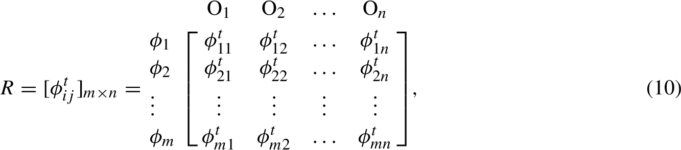 where ${\phi _{ij}^{t}}$ ($i=1,2,\dots ,m$, $j=1,2,\dots ,n$) denotes the evaluation information of alternative ${\phi _{i}}$ $(i=1,2,\dots ,m)$ with respect to attribute ${O_{j}}$ $(j=1,2,\dots ,n)$ by expert ${d^{t}}$.
Step 2.
According to some aggregation operators, we can utilize overall ${\phi _{ij}^{t}}$ to ${\phi _{ij}}$.
Step 3.
Normalize the fused results’ matrix $r={[{\phi _{ij}}]_{m\times n}}$, $i=1,2,\dots ,m$, $j=1,2,\dots ,n$ based on the type of each attributes by the following formula:
For benefit attributes:
Step 4.
According to the normalized matrix ${N_{ij}}$ ($i=1,2,\dots ,m$, $j=1,2,\dots ,n$) and attribute’s weighting vector ${w_{j}}$ $(j=1,2,\dots ,n)$, the weighted normalized matrix $W{N_{ij}}$ ($i=1,2,\dots ,m$, $j=1,2,\dots ,n$) can be computed as:
Step 5.
Step 6.
Calculate the distance $D={[{d_{ij}}]_{m\times n}}$ between each alternatives and the border approximation area (BAA) by the following equation:
where $d(W{N_{ij}},{g_{j}})$ means the distance from $W{N_{ij}}$ to ${g_{j}}$. According to the values of ${d_{ij}}$, we can get:
Obviously, the best alternatives are included in ${G^{+}}$ (UAA) and the worst alternatives are included in ${G^{-}}$ (LAA).
(15)
\[ {d_{ij}}=\left\{\begin{array}{l@{\hskip4.0pt}l}d(W{N_{ij}},{g_{j}}),\hspace{1em}& \text{if}\hspace{2.5pt}W{N_{ij}}>{g_{j}},\\ {} 0,\hspace{1em}& \text{if}\hspace{2.5pt}W{N_{ij}}={g_{j}},\\ {} -d(W{N_{ij}},{g_{j}})\hspace{1em}& \text{if}\hspace{2.5pt}W{N_{ij}}<{g_{j}},\end{array}\right.\](1)
if ${d_{ij}}>0$, the alternatives belong to the upper approximation area ${G^{+}}$ (UAA);
(2)
if ${d_{ij}}=0$, the alternatives belong to the border approximation area G (BAA);
(3)
if ${d_{ij}}<0$, the alternatives belong to the lower approximation area ${G^{-}}$ (LAA).
Step 7.
Sum the values of each alternative’s ${d_{ij}}$ with respect to all the attributes by following equation:
According to the calculating results of ${S_{i}}$,we can rank all the alternatives, the bigger the value of ${S_{i}}$ is, the better alternative will be selected.
4 The MABAC Model with 2-tuple Linguistic Neutrosophic Information
By combiningthe MABAC method with 2-tuple linguistic neutrosophic information, we can build the 2-tuple linguistic neutrosophic MABAC model where all the evaluation information and attribute’s weighting vector are presented with 2-tuple linguistic neutrosophic numbers (2TLNNs). Suppose there are m alternatives $\{{\phi _{1}},{\phi _{2}},\dots ,{\phi _{m}}\}$, n attributes $\{{O_{1}},{O_{2}},\dots ,{O_{n}}\}$ with weighting vector ${w_{j}}$ $(j=1,2,\dots ,n)$ and t experts $\{{d_{1}},{d_{2}},\dots ,{d_{t}}\}$ with weighting vector $\{{v_{1}},{v_{2}},\dots ,{v_{t}}\}$, the decision-making steps are expressed as follows.
Step 1.
Construct the 2-tuple linguistic neutrosophic evaluation matrix $R={[{\phi _{ij}^{t}}]_{m\times n}}$, $i=1,2,\dots ,m$, $j=1,2,\dots ,n$ which can be depicted as follows: 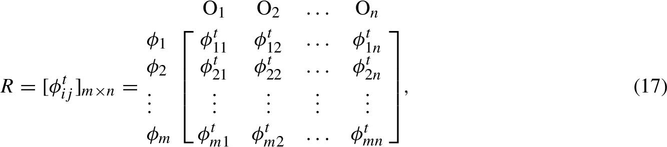 where ${\phi _{ij}^{t}}=\{{({s_{{t_{ij}}}},{\alpha _{ij}})^{t}},{({s_{{i_{ij}}}},{\beta _{ij}})^{t}},{({s_{{f_{ij}}}},{\chi _{ij}})^{t}}\}$ ($i=1,2,\dots ,m$, $j=1,2,\dots ,n$) denotes the 2-tuple linguistic neutrosophic information of alternative ${\phi _{i}}$ $(i=1,2,\dots ,m)$ on attribute ${O_{j}}$ $(j=1,2,\dots ,n)$ by expert ${d^{t}}$.
Step 2.
According to the 2TLNNWA or 2TLNNWG aggregation operators, we can utilize overall ${\phi _{ij}^{t}}$ to ${\phi _{ij}}$, the fused 2TLNNs matrix $r={[{\phi _{ij}}]_{m\times n}}$ shown as follows:  where ${\phi _{ij}}=\{({s_{{t_{ij}}}},{\alpha _{ij}}),({s_{{i_{ij}}}},{\beta _{ij}}),({s_{{f_{ij}}}},{\chi _{ij}})\}$ ($i=1,2,\dots ,m$, $j=1,2,\dots ,n$) denotes the fused 2-tuple linguistic neutrosophic information of alternative ${\phi _{i}}$ $(i=1,2,\dots ,m)$ on attribute ${O_{j}}$ $(j=1,2,\dots ,n)$.
Step 3.
Normalize the matrix $r={[{\phi _{ij}}]_{m\times n}}$, $i=1,2,\dots ,m$, $j=1,2,\dots ,n$ based on the type of each attribute by the following formula; for benefit attributes:
(19)
\[\begin{aligned}{}{N_{ij}}& ={\phi _{ij}}=\{{({s_{{t_{ij}}}},{\alpha _{ij}})^{\prime }},{({s_{{i_{ij}}}},{\beta _{ij}})^{\prime }},{({s_{{f_{ij}}}},{\chi _{ij}})^{\prime }}\}\\ {} & =\{({s_{{t_{ij}}}},{\alpha _{ij}}),({s_{{i_{ij}}}},{\beta _{ij}}),({s_{{f_{ij}}}},{\chi _{ij}})\},\\ {} & \hspace{1em}i=1,2,\dots ,m,\hspace{2.5pt}j=1,2,\dots ,n.\end{aligned}\]For cost attributes:
(20)
\[\begin{aligned}{}& {N_{ij}}=k-{\phi _{ij}}=\left\{\substack{{({s_{{t_{ij}}}},{\alpha _{ij}})^{\prime }},\\ {} {({s_{{i_{ij}}}},{\beta _{ij}})^{\prime }},\\ {} {({s_{{f_{ij}}}},{\chi _{ij}})^{\prime }}}\right\}=\left\{\substack{\Delta (k-{\Delta ^{-1}}({s_{{t_{ij}}}},{\alpha _{ij}})),\\ {} \Delta (k-{\Delta ^{-1}}({s_{{i_{ij}}}},{\beta _{ij}})),\\ {} \Delta (k-{\Delta ^{-1}}({s_{{f_{ij}}}},{\chi _{ij}}))}\right\},\\ {} & i=1,2,\dots ,m,\hspace{2.5pt}j=1,2,\dots ,n.\end{aligned}\]Step 4.
According to the normalized matrix ${N_{ij}}=\{{({s_{{t_{ij}}}},{\alpha _{ij}})^{\prime }},{({s_{{i_{ij}}}},{\beta _{ij}})^{\prime }},{({s_{{f_{ij}}}},{\chi _{ij}})^{\prime }}\}$ ($i=1,2,\dots ,m$, $j=1,2,\dots ,n$) and attribute’s weighting vector ${w_{j}}$ $(j=1,2,\dots ,n)$, the fuzzy weighted normalized matrix $W{N_{ij}}=\{{({s_{{t_{ij}}}},{\alpha _{ij}})^{\prime\prime }},{({s_{{i_{ij}}}},{\beta _{ij}})^{\prime\prime }},{({s_{{f_{ij}}}},{\chi _{ij}})^{\prime\prime }}\}$ ($i=1,2,\dots ,m$, $j=1,2,\dots ,n$) can be computed as:
(21)
\[\begin{aligned}{}W{N_{ij}}& ={w_{j}}\otimes {N_{ij}}=\big\{{({s_{{t_{ij}}}},{\alpha _{ij}})^{\prime\prime }},{({s_{{i_{ij}}}},{\beta _{ij}})^{\prime\prime }},{({s_{{f_{ij}}}},{\chi _{ij}})^{\prime\prime }}\big\}\\ {} & =\left\{\begin{array}{l}\Delta \bigg(k\bigg(1-{\bigg(1-\frac{{\Delta ^{-1}}{({s_{{t_{ij}}}},{\alpha _{ij}})^{\prime }}}{k}\bigg)^{{w_{j}}}}\bigg)\bigg),\Delta \bigg(k{\bigg(\frac{{\Delta ^{-1}}{({s_{{i_{ij}}}},{\beta _{ij}})^{\prime }}}{k}\bigg)^{{w_{j}}}}\bigg),\\ {} \Delta \bigg(k{\bigg(\frac{{\Delta ^{-1}}{({s_{{f_{ij}}}},{\chi _{ij}})^{\prime }}}{k}\bigg)^{{w_{j}}}}\bigg)\end{array}\right\}\\ {} & (i=1,2,\dots ,m,j=1,2,\dots ,n).\end{aligned}\]Step 5.
Compute the values of border approximation area (BAA) and the BAA matrix $G={[{g_{j}}]_{1\times n}}$ can be constructed as follows:
(22)
\[\begin{aligned}{}{g_{j}}& ={\bigg({\prod \limits_{i=1}^{m}}W{N_{ij}}\bigg)^{1/m}}\end{aligned}\](23)
\[\begin{aligned}{}& =\left\{\begin{array}{l}\Delta \bigg(k{\textstyle\prod \limits_{i=1}^{m}}{\bigg(\frac{{\Delta ^{-1}}{({s_{{t_{ij}}}},{\alpha _{ij}})^{\prime\prime }}}{k}\bigg)^{1/m}}\bigg),\\ {} \Delta \bigg(k\bigg(1-{\textstyle\prod \limits_{i=1}^{m}}{\bigg(1-\frac{{\Delta ^{-1}}{({s_{{i_{ij}}}},{\beta _{ij}})^{\prime\prime }}}{k}\bigg)^{1/m}}\bigg)\bigg),\\ {} \Delta \bigg(k\bigg(1-{\textstyle\prod \limits_{i=1}^{m}}{\bigg(1-\frac{{\Delta ^{-1}}{({s_{{f_{ij}}}},{\chi _{ij}})^{\prime\prime }}}{k}\bigg)^{1/m}}\bigg)\bigg)\end{array}\right\}.\end{aligned}\]Step 6.
Calculate the distance $D={[{d_{ij}}]_{m\times n}}$ between each alternatives and the border approximation area (BAA) by the following equation:
where $d(W{N_{ij}},{g_{j}})$ means the distance from $W{N_{ij}}$ to ${g_{j}}$.
(24)
\[ {d_{ij}}=\left\{\begin{array}{l@{\hskip4.0pt}l}d(W{N_{ij}},{g_{j}}),\hspace{1em}& \text{if}\hspace{2.5pt}W{N_{ij}}>{g_{j}},\\ {} 0,\hspace{1em}& \text{if}\hspace{2.5pt}W{N_{ij}}={g_{j}},\\ {} -d(W{N_{ij}},{g_{j}})\hspace{1em}& \text{if}\hspace{2.5pt}W{N_{ij}}<{g_{j}},\end{array}\right.\]Step 7.
Sum the values of each alternative’s with respect to all the attributes by the following equation:
According to the calculation results of ${S_{i}}$,we can rank all the alternatives, the bigger the value of ${S_{i}}$ is, the better alternative will be selected.
5 The Numerical Example
5.1 Numerical Example for 2TLNNs MAGDM Problems
If the construction enterprise wants to be in a good position in the new round of competition in the market, it must adapt to the changing market competition environment. In order to increase their core competitiveness, the effective method is the low cost strategy. When analysing the cost control of the construction project, it is found that there are many problems in the current cost control, especially the cost control methods are backward and rough, and the empirical elements are too many, and there is no credible basis. If you can’t carry out an effective cost control, the prospects are predictable. Therefore, it is very important to develop and improve the cost control methods of construction projects to enhance the core competitiveness of enterprises. In order to select the best construction projects classical MADM problems are helpful (Li et al., 2018a, 2018b; Wang et al., 2019a, 2019b; Wei, 2019; Wei and Zhang, 2019; Zhang et al., 2019). In this section, we provide a numerical example to select the best construction projects by using MABAC model with 2-tuple linguistic neutrosophic information. Assume that five possible construction projects ${\phi _{i}}$ $(i=1,2,3,4,5)$ are to be selected and four attributes to assess these construction projects: (1) ${O_{1}}$ is the human factor in construction projects; (2) ${O_{2}}$ is the energy cost factor; (3) ${O_{3}}$ is the building materials and equipment factor; (4) ${O_{4}}$ is the environmental factor. The five possible construction projects ${\phi _{i}}$ ($i=1,2,3,4,5$) are to be evaluated with 2TLNNs with the four criteria by three experts ${d^{t}}$ (Suppose expert’s weighting vector is $(0.3,0.4,0.3)$ and attribute’s weighting vector is $(0.4,0.1,0.3,0.2)$).
Step 1.
Construct the 2-tuple linguistic neutrosophic evaluation matrix $R={[{\phi _{ij}^{t}}]_{m\times n}}$, $i=1,2,\dots ,m$, $j=1,2,\dots ,n$.
Table 1
2-tuple linguistic neutrosophic evaluation information by ${d^{1}}$.
| ${O_{1}}$ | ${O_{2}}$ | |
| ${\phi _{1}}$ | $\{({s_{2}},0),({s_{3}},0),({s_{4}},0)\}$ | $\{({s_{4}},0),({s_{3}},0),({s_{1}},0)\}$ |
| ${\phi _{2}}$ | $\{({s_{5}},0),({s_{1}},0),({s_{1}},0)\}$ | $\{({s_{5}},0),({s_{2}},0),({s_{1}},0)\}$ |
| ${\phi _{3}}$ | $\{({s_{2}},0),({s_{3}},0),({s_{1}},0)\}$ | $\{({s_{4}},0),({s_{2}},0),({s_{3}},0)\}$ |
| ${\phi _{4}}$ | $\{({s_{4}},0),({s_{5}},0),({s_{4}},0)\}$ | $\{({s_{3}},0),({s_{4}},0),({s_{3}},0)\}$ |
| ${\phi _{5}}$ | $\{({s_{1}},0),({s_{1}},0),({s_{4}},0)\}$ | $\{({s_{2}},0),({s_{1}},0),({s_{5}},0)\}$ |
| ${O_{3}}$ | ${O_{4}}$ | |
| ${\phi _{1}}$ | $\{({s_{2}},0),({s_{4}},0),({s_{3}},0)\}$ | $\{({s_{1}},0),({s_{3}},0),({s_{2}},0)\}$ |
| ${\phi _{2}}$ | $\{({s_{4}},0),({s_{1}},0),({s_{2}},0)\}$ | $\{({s_{5}},0),({s_{3}},0),({s_{4}},0)\}$ |
| ${\phi _{3}}$ | $\{({s_{4}},0),({s_{2}},0),({s_{5}},0)\}$ | $\{({s_{3}},0),({s_{2}},0),({s_{1}},0)\}$ |
| ${\phi _{4}}$ | $\{({s_{2}},0),({s_{4}},0),({s_{1}},0)\}$ | $\{({s_{4}},0),({s_{5}},0),({s_{2}},0)\}$ |
| ${\phi _{5}}$ | $\{({s_{3}},0),({s_{1}},0),({s_{5}},0)\}$ | $\{({s_{2}},0),({s_{2}},0),({s_{4}},0)\}$ |
Table 2
2-tuple linguistic neutrosophic evaluation information by ${d^{2}}$.
| ${O_{1}}$ | ${O_{2}}$ | |
| ${\phi _{1}}$ | $\{({s_{3}},0),({s_{2}},0),({s_{5}},0)\}$ | $\{({s_{2}},0),({s_{4}},0),({s_{5}},0)\}$ |
| ${\phi _{2}}$ | $\{({s_{5}},0),({s_{2}},0),({s_{3}},0)\}$ | $\{({s_{5}},0),({s_{2}},0),({s_{3}},0)\}$ |
| ${\phi _{3}}$ | $\{({s_{4}},0),({s_{3}},0),({s_{2}},0)\}$ | $\{({s_{5}},0),({s_{1}},0),({s_{2}},0)\}$ |
| ${\phi _{4}}$ | $\{({s_{3}},0),({s_{2}},0),({s_{5}},0)\}$ | $\{({s_{1}},0),({s_{5}},0),({s_{2}},0)\}$ |
| ${\phi _{5}}$ | $\{({s_{2}},0),({s_{2}},0),({s_{3}},0)\}$ | $\{({s_{2}},0),({s_{3}},0),({s_{4}},0)\}$ |
| ${O_{3}}$ | ${O_{4}}$ | |
| ${\phi _{1}}$ | $\{({s_{5}},0),({s_{2}},0),({s_{1}},0)\}$ | $\{({s_{2}},0),({s_{4}},0),({s_{3}},0)\}$ |
| ${\phi _{2}}$ | $\{({s_{4}},0),({s_{3}},0),({s_{1}},0)\}$ | $\{({s_{4}},0),({s_{2}},0),({s_{1}},0)\}$ |
| ${\phi _{3}}$ | $\{({s_{1}},0),({s_{2}},0),({s_{4}},0)\}$ | $\{({s_{2}},0),({s_{4}},0),({s_{5}},0)\}$ |
| ${\phi _{4}}$ | $\{({s_{5}},0),({s_{2}},0),({s_{3}},0)\}$ | $\{({s_{2}},0),({s_{4}},0),({s_{3}},0)\}$ |
| ${\phi _{5}}$ | $\{({s_{2}},0),({s_{1}},0),({s_{5}},0)\}$ | $\{({s_{2}},0),({s_{3}},0),({s_{4}},0)\}$ |
Table 3
2-tuple linguistic neutrosophic evaluation information by ${d^{3}}$.
| ${O_{1}}$ | ${O_{2}}$ | |
| ${\phi _{1}}$ | $\{({s_{2}},0),({s_{1}},0),({s_{4}},0)\}$ | $\{({s_{1}},0),({s_{3}},0),({s_{5}},0)\}$ |
| ${\phi _{2}}$ | $\{({s_{4}},0),({s_{1}},0),({s_{2}},0)\}$ | $\{({s_{5}},0),({s_{2}},0),({s_{1}},0)\}$ |
| ${\phi _{3}}$ | $\{({s_{5}},0),({s_{4}},0),({s_{4}},0)\}$ | $\{({s_{2}},0),({s_{5}},0),({s_{4}},0)\}$ |
| ${\phi _{4}}$ | $\{({s_{5}},0),({s_{3}},0),({s_{4}},0)\}$ | $\{({s_{1}},0),({s_{4}},0),({s_{3}},0)\}$ |
| ${\phi _{5}}$ | $\{({s_{1}},0),({s_{2}},0),({s_{4}},0)\}$ | $\{({s_{4}},0),({s_{2}},0),({s_{3}},0)\}$ |
| ${O_{3}}$ | ${O_{4}}$ | |
| ${\phi _{1}}$ | $\{({s_{3}},0),({s_{4}},0),({s_{2}},0)\}$ | $\{({s_{3}},0),({s_{5}},0),({s_{2}},0)\}$ |
| ${\phi _{2}}$ | $\{({s_{4}},0),({s_{1}},0),({s_{2}},0)\}$ | $\{({s_{5}},0),({s_{3}},0),({s_{2}},0)\}$ |
| ${\phi _{3}}$ | $\{({s_{3}},0),({s_{2}},0),({s_{5}},0)\}$ | $\{({s_{1}},0),({s_{3}},0),({s_{4}},0)\}$ |
| ${\phi _{4}}$ | $\{({s_{2}},0),({s_{4}},0),({s_{1}},0)\}$ | $\{({s_{3}},0),({s_{5}},0),({s_{2}},0)\}$ |
| ${\phi _{5}}$ | $\{({s_{2}},0),({s_{3}},0),({s_{4}},0)\}$ | $\{({s_{4}},0),({s_{2}},0),({s_{1}},0)\}$ |
Step 2.
Then according to 2TLNNWA operator and expert’s weighting vector, we can utilize overall ${\phi _{ij}^{t}}$ to ${\phi _{ij}}$ to obtain the matrix $r={[{\phi _{ij}}]_{m\times n}}$, $i=1,2,\dots ,m$, $j=1,2,\dots ,n$ as follows.
Table 4
The aggregation results by 2TLNNWA operator.
| ${O_{1}}$ | ${O_{2}}$ | |
| ${\phi _{1}}$ | $\{({s_{2}},0.4348),({s_{2}},-0.1654),({s_{4}},0.3734)\}$ | $\{({s_{3}},-0.4740),({s_{3}},0.3659),({s_{3}},0.0852)\}$ |
| ${\phi _{2}}$ | $\{({s_{5}},-0.2311),({s_{1}},03195),({s_{2}},-0.0895)\}$ | $\{({s_{1}},0.4269),({s_{2}},0.3522),({s_{5}},0.0000)\}$ |
| ${\phi _{3}}$ | $\{({s_{4}},0.0000),({s_{3}},0.2704),({s_{2}},0.0000)\}$ | $\{({s_{4}},0.1339),({s_{2}},-0.0047),({s_{3}},-0.2192)\}$ |
| ${\phi _{4}}$ | $\{({s_{4}},0.0895),({s_{3}},-0.0267),({s_{4}},0.3734)\}$ | $\{({s_{2}},-0.2896),({s_{4}},0.3734),({s_{3}},-0.4492)\}$ |
| ${\phi _{5}}$ | $\{({s_{1}},0.4269),({s_{2}},-0.3755),({s_{4}},-0.4348)\}$ | $\{({s_{3}},-0.2490),({s_{2}},-0.0895),({s_{4}},-0.0767)\}$ |
| ${O_{3}}$ | ${O_{4}}$ | |
| ${\phi _{1}}$ | $\{({s_{4}},-0.1074),({s_{3}},0.0314),({s_{2}},-0.2882)\}$ | $\{({s_{2}},0.0767),({s_{4}},-0.0767),({s_{2}},0.3522)\}$ |
| ${\phi _{2}}$ | $\{({s_{4}},0.0000),({s_{2}},-0.4482),({s_{2}},-0.4843)\}$ | $\{({s_{5}},-0.3195),({s_{3}},-0.4492),({s_{2}},-0.1339)\}$ |
| ${\phi _{3}}$ | $\{({s_{3}},-0.2586),({s_{2}},0.0000),({s_{5}},-0.4269)\}$ | $\{({s_{2}},0.0767),({s_{3}},-0.0196),({s_{3}},-0.1146)\}$ |
| ${\phi _{4}}$ | $\{({s_{4}},-0.2974),({s_{3}},0.0314),({s_{2}},-0.4482)\}$ | $\{({s_{3}},0.0196),({s_{5}},-0.4269),({s_{2}},0.3522)\}$ |
| ${\phi _{5}}$ | $\{({s_{2}},0.3307),({s_{1}},0.3904),({s_{5}},-0.3238)\}$ | $\{({s_{3}},-0.2490),({s_{2}},0.3522),({s_{3}},-0.3610)\}$ |
Step 3.
Normalize the fused results matrix $r={[{\phi _{ij}}]_{m\times n}}$, $i=1,2,\dots ,m$, $j=1,2,\dots ,n$ based on the type of each attributes by formula (19) and (20); (O2 is the cost attribute).
Table 5
The normalized decision-making matrix ${N_{ij}}$.
| ${O_{1}}$ | ${O_{2}}$ | |
| ${\phi _{1}}$ | $\{({s_{2}},0.4348),({s_{2}},-0.1654),({s_{4}},0.3734)\}$ | $\{({s_{3}},0.4740),({s_{3}},-0.3659),({s_{3}},-0.0852)\}$ |
| ${\phi _{2}}$ | $\{({s_{5}},-0.2311),({s_{1}},0.3195),({s_{2}},-0.0895)\}$ | $\{({s_{5}},-0.4269),({s_{4}},-0.3522),({s_{1}},0.0000)\}$ |
| ${\phi _{3}}$ | $\{({s_{4}},0.0000),({s_{3}},0.2704),({s_{2}},0.0000)\}$ | $\{({s_{2}},-0.1339),({s_{4}},0.0047),({s_{3}},0.2192)\}\hspace{2.5pt}$ |
| ${\phi _{4}}$ | $\{({s_{4}},0.0895),({s_{3}},-0.2367),({s_{4}},0.3734)\}$ | $\{({s_{4}},0.2896),({s_{2}},-0.3734),({s_{3}},0.4492)\}\hspace{2.5pt}$ |
| ${\phi _{5}}$ | $\{({s_{1}},0.4269),({s_{2}},-0.3755),({s_{4}},-0.4348)\}$ | $\{({s_{3}},0.2490),({s_{4}},0.0895),({s_{2}},0.0767)\}$ |
| ${O_{3}}$ | ${O_{4}}$ | |
| ${\phi _{1}}$ | $\{({s_{4}},-0.1074),({s_{3}},0314),({s_{2}},-0.2882)\}$ | $\{({s_{2}},0767),({s_{4}},-0.0767),({s_{2}},0.3522)\}$ |
| ${\phi _{2}}$ | $\{({s_{4}},0.0000),({s_{2}},-0.4482),({s_{2}},-0.4843)\}$ | $\{({s_{5}},-0.3195),({s_{3}},-0.4492),({s_{2}},-0.1339)\}$ |
| ${\phi _{3}}$ | $\{({s_{3}},-0.2586),({s_{2}},0.0000),({s_{5}},-0.4269)\}$ | $\{({s_{2}},0.0767),({s_{3}},-0.0196),({s_{3}},-0.1146)\}$ |
| ${\phi _{4}}$ | $\{({s_{4}},-0.2974),({s_{3}},0.0314),({s_{2}},-0.4482)\}$ | $\{({s_{3}},0.0196),({s_{5}},-0.4269),({s_{2}},0.3522)\}$ |
| ${\phi _{5}}$ | $\{({s_{2}},0.3307),({s_{1}},0.3904),({s_{5}},-0.3238)\}$ | $\{({s_{3}},-0.2490),({s_{2}},0.3522),({s_{3}},-0.3610)\}$ |
Step 4.
According to the normalized matrix ($i=1,2,\dots ,m$, $j=1,2,\dots ,n$) and attribute’s weighting vector ${w_{j}}$ $(j=1,2,\dots ,n)$, the weighted normalized matrix $W{N_{ij}}$, $i=1,2,\dots ,m$, $j=1,2,\dots ,n$ can be computed as:
Table 6
Weighted normalized average matrix $W{N_{ij}}$.
| ${O_{1}}$ | ${O_{2}}$ | |
| ${\phi _{1}}$ | $\{({s_{1}},0.1278),({s_{4}},-0.2648),({s_{5}},0.2871)\}$ | $\{({s_{0}},0.4972),({s_{6}},-0.4741),({s_{6}},-0.4179)\}$ |
| ${\phi _{2}}$ | $\{({s_{3}},-0.1843),({s_{3}},0.2738),({s_{4}},-0.2038)\}$ | $\{({s_{1}},-0.1973),({s_{6}},-0.2913),({s_{5}},0.0158)\}$ |
| ${\phi _{3}}$ | $\{({s_{2}},0.1336),({s_{5}},-0.2931),({s_{4}},-0.1336)\}$ | $\{({s_{0}},0.2194),({s_{6}},-0.2377),({s_{2}},3622)\}$ |
| ${\phi _{4}}$ | $\{({s_{2}},0.2038),({s_{5}},-0.4691),({s_{5}},0.2871)\}$ | $\{({s_{1}},-0.2923),({s_{5}},0.2658),({s_{6}},-0.3232)\}$ |
| ${\phi _{5}}$ | $\{({s_{1}},-0.3824),({s_{4}},-0.4422),({s_{5}},-0.1278)\}$ | $\{({s_{0}},0.4501),({s_{6}},-0.2257),({s_{5}},0.3960)\}$ |
| ${O_{3}}$ | ${O_{4}}$ | |
| ${\phi _{1}}$ | $\{({s_{3}},-0.3836),({s_{5}},-0.1112),({s_{4}},0.1185)\}$ | $\{({s_{0}},0.4887),({s_{6}},-0.4887),({s_{5}},-0.0248)\}$ |
| ${\phi _{2}}$ | $\{({s_{2}},-0.3153),({s_{4}},-0.0009),({s_{4}},-0.0291)\}$ | $\{({s_{2}},-0.4320),({s_{5}},0.0566),({s_{5}},0.2499)\}$ |
| ${\phi _{3}}$ | $\{({s_{1}},0.0041),({s_{4}},0.3153),({s_{6}},-0.4695)\}$ | $\{({s_{0}},0.4887),({s_{5}},0.2164),({s_{5}},0.1828)\}$ |
| ${\phi _{4}}$ | $\{({s_{2}},-0.4986),({s_{5}},-0.1112),({s_{4}},-0.0009)\}$ | $\{({s_{1}},-0.2164),({s_{6}},-0.3172),({s_{5}},-0.0248)\}$ |
| ${\phi _{5}}$ | $\{({s_{1}},-0.1770),({s_{4}},-0.1306),({s_{6}},-0.4323)\}$ | $\{({s_{1}},-0.3073),({s_{5}},-0.0248),({s_{5}},0.0911)\}$ |
Step 5.
Compute the values of border approximation area (BAA) and the BAA matrix $G={[{g_{j}}]_{1\times n}}$ can be constructed as follows:
\[\begin{aligned}{}& {g_{1}}=\{({s_{2}},-1.6327)({s_{4}},-3.2448),({s_{5}},-4.1188)\},\\ {} & {g_{2}}=\{({s_{0}},0.1179,)({s_{6}},-5.1224),({s_{6}},-5.0539)\},\\ {} & {g_{3}}=\{({s_{1}},-0.7498)({s_{4}},-3.1852),({s_{5}},-4.3335)\},\\ {} & {g_{4}}=\{({s_{1}},-0.8694),({s_{5}},-4.0529),({s_{5}},-4.1708)\}.\end{aligned}\]
Step 6.
Calculate the distance $D={[{d_{ij}}]_{m\times n}}$ between each alternatives and the border approximation area (BAA) by equation (23).
Table 7
The distances between ${d_{ij}}$ alternatives and BAA.
| ${O_{1}}$ | ${O_{2}}$ | ${O_{3}}$ | ${O_{4}}$ | |
| ${\phi _{1}}$ | $\{-0.0693\}$ | $\{0.0114\}$ | $\{0.0870\}$ | $\{-0.0239\}$ |
| ${\phi _{2}}$ | $\{0.1673\}$ | $\{0.0481\}$ | $\{0.1000\}$ | $\{0.0771\}$ |
| ${\phi _{3}}$ | $\{0.1195\}$ | $\{-0.0286\}$ | $\{-0.0573\}$ | $\{-0.0305\}$ |
| ${\phi _{4}}$ | $\{-0.0910\}$ | $\{0.0428\}$ | $\{0.0873\}$ | $\{-0.0234\}$ |
| ${\phi _{5}}$ | $\{-0.0844\}$ | $\{-0.0154\}$ | $\{-0.0942\}$ | $\{0.0274\}$ |
Step 7.
Sum the values of each alternative’s ${d_{ij}}$ with respect to all the attributes by equation (24);
\[ {S_{1}}=0.0052,\hspace{1em}{S_{2}}=0.3925,\hspace{1em}{S_{3}}=0.0032,\hspace{1em}{S_{4}}=0.0157,\hspace{1em}{S_{5}}=-0.1665.\]
According to the calculating results of ${S_{i}}$,we can rank all the alternatives, the bigger the value of ${S_{i}}$ is, the better alternative will be selected. Obviously, the rank of all alternatives is ${\phi _{2}}>{\phi _{4}}>{\phi _{1}}>{\phi _{3}}>{\phi _{5}}$ and ${\phi _{2}}$ is the best alternative.5.2 Comparison of 2TLNNs MABAC Method with Some 2TLNNs Aggregation Operators
In this chapter, we compare our proposed 2-tuple linguistic neutrosophic MABAC method with the 2-tuple linguistic neutrosophic weighted average (2TLNNWA) operator and the 2-tuple linguistic neutrosophic weighted geometric (2TLNNWG) operator (Wu et al., 2018b). Based on the attribute’s weight and results of Table 4, the fused values by 2TLNNWA and 2TLNNWG operators are shown in Table 8.
Table 8
The fused values by using some 2TLNNs aggregation operator.
| 2TLNNWA | 2TLNNWG | |
| ${\phi _{1}}$ | $\{({s_{3}},-0.3685),({s_{3}},-0.3615),({s_{3}},-0.1843)\}$ | $\{({s_{3}},-0.2749),({s_{3}},-0.1273),({s_{3}},0.2894)\}$ |
| ${\phi _{2}}$ | $\{({s_{4}},-0.1286),({s_{2}},-0.3254),({s_{2}},-0.0469)\}$ | $\{({s_{4}},-0.0053),({s_{2}},-0.2298),({s_{2}},0.3403)\}$ |
| ${\phi _{3}}$ | $\{({s_{3}},-0.1443),({s_{3}},-0.3636),({s_{3}},-0.1494)\}$ | $\{({s_{3}},0.1429),({s_{3}},-0.2457),({s_{3}},0.2672)\}$ |
| ${\phi _{4}}$ | $\{({s_{3}},0.1191),({s_{3}},0.3878),({s_{3}},-0.3175)\}$ | $\{({s_{3}},0.4239),({s_{4}},-0.4331),({s_{3}},0.2130)\}$ |
| ${\phi _{5}}$ | $\{({s_{2}},-0.0375),(s2,-0.3032),({s_{4}},-0.3233)\}$ | $\{(s2,0.0131),(s2,-0.2568),({s_{4}},-0.1289)\}$ |
According to the score function of 2TLNNs, we can obtain the alternative score results which are shown in Table 9.
Table 9
Score results of alternatives ${\phi _{i}}$.
| 2TLNNWA | 2TLNNWG | |
| $s({\phi _{1}})$ | 0.6663 | 0.6585 |
| $s({\phi _{2}})$ | 0.7877 | 0.7902 |
| $s({\phi _{3}})$ | 0.6789 | 0.6883 |
| $s({\phi _{4}})$ | 0.6517 | 0.6587 |
| $s({\phi _{5}})$ | 0.6814 | 0.6817 |
The ranking of alternatives by some 2TLNNs aggregation operators are listed as follows.
Table 10
Rank of alternatives by some 2TLNNs aggregation operators.
| Order | |
| 2TLNNWA | $\{{\phi _{2}}>{\phi _{5}}>{\phi _{3}}>{\phi _{1}}>{\phi _{4}}\}$ |
| 2TLNNWG | $\{{\phi _{2}}>{\phi _{3}}>{\phi _{5}}>{\phi _{4}}>{\phi _{1}}\}$ |
| 2TLNNs MABAC model | $\{{\phi _{2}}>{\phi _{4}}>{\phi _{1}}>{\phi _{3}}>{\phi _{5}}\}$ |
Comparing the results of the 2-tuple linguistic neutrosophic MABAC model with 2TLNNWA and 2TLNNWG operators, the aggregation results are slightly different in ranking of alternatives and the best alternatives are same. However, 2-tuple linguistic neutrosophic MABAC model has the unique characteristics of computing the distance between each alternatives and the border approximation area (BAA) and can be more accurate and effective in the application of MADM problems.
6 Conclusions
In this paper, we present the 2-tuple linguistic neutrosophic MABAC model based on the traditional MABAC (multi-attributive border approximation area comparison) model and some fundamental theories of 2-tuple linguistic neutrosophic information. Firstly, we briefly review the definition of 2-tuple linguistic neutrosophic sets (2TLNNSs) and introduce the score function, accuracy function, operation laws and some aggregation operators of 2TLNNs. Then, the calculation steps of traditional MABAC model are briefly presented. Furthermore, by combining the traditional MABAC model with 2TLNNs information, the 2-tuple linguistic neutrosophic MABAC model is established and the computing steps are simply depicted. Our presented model is more accurate and effective for computing the distance between each alternatives and the border approximation area (BAA). Finally, a numerical example for safety assessment of construction project has been given to illustrate this new model and some comparisons between 2TLNNs MABAC model and two 2TLNNs aggregation operators are also made to further illustrate the advantages of the new method. In the future, the 2-tuple linguistic neutrosophic MABAC model can be applied to the risk analysis (Khraisha and Arthur, 2018; Lenka and Barik, 2018; Wei et al., 2017, 2018f), the MADM problems (Dong et al., 2018; Kou et al., 2016; Mardani et al., 2018; Morente-Molinera et al., 2018; Sremac et al., 2018) and many other uncertain and fuzzy environments (Ghorabaee et al., 2017; Peng et al., 2018; Peng and Garg, 2018; Peng and Yang, 2017; Peng et al., 2017b; Wei and Gao, 2018; Wei et al., 2018a, 2018b, 2018c, 2018d, 2018e; Wei et al., 2019; Wei and Wei, 2018b)


