Informatica logo


Login Register

  1. Home
  2. Issues
  3. Volume 30, Issue 3 (2019)
  4. An Effective Hybrid Fuzzy Programming Ap ...

Informatica

Information Submit your article For Referees Help ATTENTION!
  • Article info
  • Full article
  • Cited by
  • More
    Article info Full article Cited by

An Effective Hybrid Fuzzy Programming Approach for an Entropy-Based Multi-Objective Assembly Line Balancing Problem
Volume 30, Issue 3 (2019), pp. 503–528
Ali Mahmoodirad   Ahmad Heydari   Sadegh Niroomand  

Authors

 
Placeholder
https://doi.org/10.15388/Informatica.2019.216
Pub. online: 1 January 2019      Type: Research Article      Open accessOpen Access

Received
1 March 2018
Accepted
1 March 2019
Published
1 January 2019

Abstract

In cases where the balance problem of an assembly line with the aim to distribute the work loads among the stations as equal as possible, the concept of entropy function can be used. In this paper, a typical assembly line balancing problem with different objective functions such as entropy-based objective function plus two more objective functions like equipment purchasing cost and worker time-dependent wage is formulated. The non-linear entropy-based objective function is approximated as a linear function using the bounded variable method of linear programming. A new hybrid fuzzy programming approach is proposed to solve the proposed multi-objective formulation efficiently. The extensive computational experiments on some test problems proves the efficiency of the proposed solution approach comparing to the available approaches of the literature.

1 Introduction

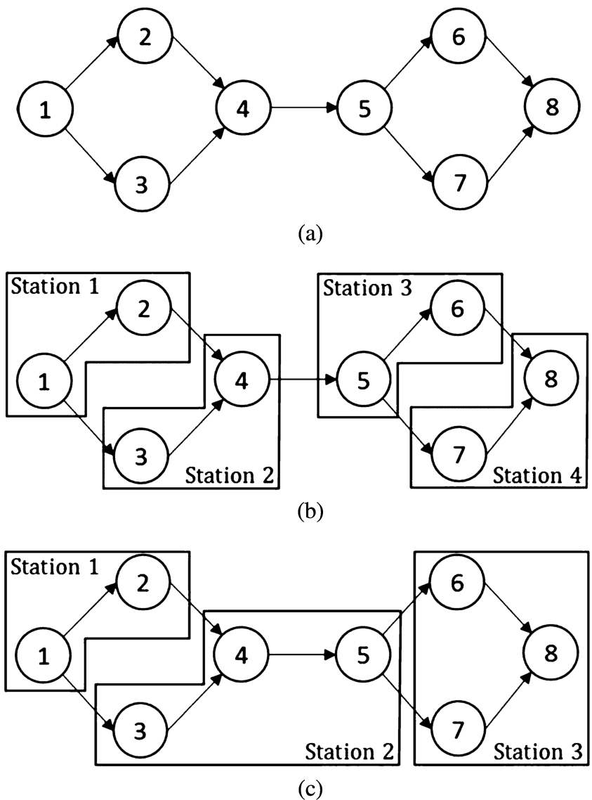
In recent competitive industrial environment, a manufacturer should be able to produce qualitative products with on-time delivery to the customers. So, designing a manufacturing environment including production department, machines’ layout, etc. is an important issue to reach the goals like better quality and on-time delivery. An effective way to have such design is to establish and balance a production (assembly) line. An assembly line consists of some tasks to be performed in a given order for producing the final product. The order of tasks is determined according to their precedence graph which defines the relationships among the tasks. The line is balanced when the tasks are assigned to some stations in order to optimize a given criterion (or a set of criteria). The stations are usually connected with a conveyor and the parts and semi-products are moved among the stations on the conveyor to be completed at the end of the line. In a balanced line each station consists of one or more tasks to be operated by usually one (in some cases more than one) worker in a given common time for all stations called cycle time of the line. The cycle time forces the line to send out a product from its last station in each cycle time. The order of stations and assigning the tasks to them must be determined in a way that would respect the precedence relationships of the tasks (precedence graph). The usual criteria used in an optimization problem of an assembly line balancing can be cycle time minimization, number of stations minimization, equipment purchasing cost minimization, worker-related cost minimization, etc. As a line balancing problem, one or more than one of these criteria may be considered for an assembly line. As an instance given by Fig. 1, assuming an assembly line which contains 8 tasks, the precedence relationships among the tasks are shown by graph (a). In this figure, the graphs (b) and (c) represent two feasible solutions which assign the tasks to 4 and 3 stations, respectively.
info1219_g001.jpg
Fig. 1
A graphical illustration of input (a) and output (b and c) for a simple assembly line balancing problem.
Assembly lines are classified from different aspects. From a physical point of view, a line can have different shapes. A line can have a straight shape if there is enough straight available space. On the other hand, it can be a U-shaped line in case of small available spaces (Baybars, 1986). Moreover, the stations may be placed on one or both sides of any assembly line. As another physical issue, the use of parallel stations may be of interest for the cases when there is a task with operating time longer than the cycle time of the line. From product variety point of view, a line can be designed to produce one type product (single model) or to produce more than one type of products (mixed-model). As another classification, a line can be designed to employ one worker in each station or to employ more than one worker in each station.
Although the literature of assembly line balancing problem is full of interesting studies, only some of its most recent studies are reported here. Lea and Gub (2016) studied a two-sided assembly line balancing problem for cycle time minimization purpose. Yuguang et al. (2016) applied a PSO meta-heuristic algorithm for a typical multi-objective hull assembly line balancing problem to minimize the goals like cycle time, static load balancing between workstations, dynamic load balancing in all workstations, and multi-station associated complexity. Sepahi and Jalali Naini (2016) modelled a two-sided assembly line balancing problem considering parallel performance of tasks. A typical two-sided assembly line balancing problem (see also Tuncel and Aydin, 2014) with mixed-model products (see also Kucukkoc and Zhang, 2014; Ramezanian and Ezzatpanah, 2015; Yang and Gao, 2016) was studied by Kucukkoc and Zhang (2016) where they used a flexible agent-based ant colony optimization solution approach. Buyukozkan et al. (2016) applied artificial bee colony and tabu search meta-heuristic approaches for a typical two-sided assembly line balancing problem. As an interesting field of assembly line balancing problems, the number of U-shaped line related studies has increased recently (see Ogan and Azizoglu, 2015; Fattahi and Turkay, 2015; Hazır and Dolgui, 2015; Alavidoost et al., 2016). Moreover, multi-objective assembly line balancing problems in certain and uncertain environments have been of interest by the studies such as Alavidoost et al. (2015), Alavidoost et al. (2016), Samouei et al. (2016), Zacharia and Th. Nearchou A. C (2016), etc. In addition to these studies, Salehi et al. (2018) considered a multi-objective assembly line balancing problem with worker’s skill and qualification considerations in fuzzy environment. Mardani-Fard et al. (2018) considered a multi-objective straight assembly line balancing problem with stochastic parameters. As an interesting problem, ergonomic issues of workers was considered in assembly line balancing problems by Battini et al. (2015) while the robotic type assembly lines were considered by Pereira and Álvarez-Miranda (2018), Borba et al. (2018), etc. For more applications of multi-objective optimization in engineering and non-engineering topics the studies of Kovács and Marian (2002), Jablonsky (2007), Tavana et al. (2014a), Hajipour et al. (2016), Zeng et al. (2016), etc. can be referred.
In this study, as a new assembly line balancing problem, an entropy-based objective function plus equipment purchasing cost and worker time-dependent wage are considered to be optimized simultaneously in an assembly line. The entropy-based non-linear objective function is linearized using a bounded variable technique which gives a good approximation of the non-linear function. As a multi-objective problem (Jablonsky, 2014; Tavana et al., 2014a; Zeng et al., 2015; Tavana et al., 2016), we propose a new hybrid fuzzy programming solution approach which has a superior performance comparing to the existing methods of the literature in the case of the problem of this study.
The rest of this paper is organized as follows. Section 2 proposes the new multi-objective assembly line balancing formulation. Section 3 describes the new solution approach proposed for the formulation of Section 2. A very detailed computational experiments are performed in Section 4. Finally, the paper ends with conclusion in Section 5.

2 Multi-Objective Entropy-Based Assembly Line Balancing Problem

The assembly line considered in this study is a straight assembly line. In this type of assembly lines the stations are arranged on a straight line, so a space with enough length should be available. Any solution for this straight assembly line balancing problem must satisfy the following general conditions:
  • • The precedence relationships among the tasks have to be satisfied among the stations too,
  • • The summation of task times of any station should not be greater than a given cycle time of the line.
Of course, some other conditions should be considered that will be explained in the mathematical model of the problem. The problem first is formulated as a non-linear multi-objective mathematical model and then is linearized as a mixed integer linear multi-objective formulation.

2.1 Non-Linear Formulation

The proposed entropy-based assembly line balancing problem of this paper uses the above-mentioned concepts to optimize an entropy objective function and two more objective functions simultaneously. In order to further formulate this problem, we need to define some notations in Table 1.
Table 1
Notationsused for mathematical formulations.
Notation Type Definition
$i(j)(I)$ Index/parameter index used for task (index used for task) (the number of tasks)
$k(r)(K)$ Index/parameter index used for station (index used for station) (the number of stations)
${t_{i}}$ Parameter processing time of task i
${\mathit{PR}_{i}}$ Parameter predecessor set of task i
${\mathit{SC}_{i}}$ Parameter successor set of task i
$\mathrm{CT}$ Variable cycle time
${X_{ik}}$ Variable 1, if task i is assigned to station k; 0, otherwise
Before constructing the whole model, the objective functions of the model are individually explained and formulated here.
Entropy maximization. In the assembly line considered in this paper, the number of stations and the cycle time value are predetermined. Each station has one worker, and the workers are assumed to be identical. The workers are paid by monthly fixed salary. Therefore, it can be of favour to distribute the tasks among the stations as equally as possible. Meaning that the sum of task times of the stations should be close to each other. For this aim the following Shannon entropy (Shannon, 1948) function can be used. This function previously has been used as the objective function of transportation problems (Ojha et al., 2009) and other optimization problems (Sun et al., 2017).
(1)
\[ \mathit{En}(Y)=-\sum \limits_{y}f(r),\]
where $p(r)$ is the probability that R is in the state of r. And, $f(r)$ is defined as follows:
(2)
\[ f(r)=\left\{\begin{array}{l@{\hskip4.0pt}l}p(r)\ln (p(r))\hspace{1em}& \text{if}\hspace{2.5pt}p(r)\ne 0,\\ {} 0\hspace{1em}& \text{if}\hspace{2.5pt}p(r)=0.\end{array}\right.\]
In assembly line problems, by normalizing the total task times of each station by the sum of all task times, the $p(r)={\textstyle\sum _{i=1}^{I}}{t_{i}}{X_{ik}}/{\textstyle\sum _{i=1}^{I}}{t_{i}}$ value for each station can be defined. Therefore, the entropy value of an assembly line can be formulated as
(3)
\[ \mathit{En}(Y)=-{\sum \limits_{k=1}^{K}}\Bigg({\sum \limits_{i=1}^{I}}{t_{i}}{X_{ik}}\Big/{\sum \limits_{i=1}^{I}}{t_{i}}\Bigg)\Bigg(\ln \Bigg({\sum \limits_{i=1}^{I}}{t_{i}}{X_{ik}}\Big/{\sum \limits_{i=1}^{I}}{t_{i}}\Bigg)\Bigg).\]
In assembly lines, the above-mentioned entropy value can be a measure of dispersal of tasks among stations. Therefore, it would be useful to use the following objective function in the proposed assembly line balancing problem.
(4)
\[ \max -{\sum \limits_{k=1}^{K}}\Bigg({\sum \limits_{i=1}^{I}}{t_{i}}{X_{ik}}\Big/{\sum \limits_{i=1}^{I}}{t_{i}}\Bigg)\Bigg(\ln \Bigg({\sum \limits_{i=1}^{I}}{t_{i}}{X_{ik}}\Big/{\sum \limits_{i=1}^{I}}{t_{i}}\Bigg)\Bigg).\]
This objective function can be converted to the following nonlinear model,
(5)
\[\begin{aligned}{}& \min {\sum \limits_{k=1}^{K}}\Bigg({\sum \limits_{i=1}^{I}}{t_{i}}{X_{ik}}\Big/{\sum \limits_{i=1}^{I}}{t_{i}}\Bigg)\Bigg(\ln \Bigg({\sum \limits_{i=1}^{I}}{t_{i}}{X_{ik}}\Big/{\sum \limits_{i=1}^{I}}{t_{i}}\Bigg)\Bigg)\end{aligned}\]
(6)
\[\begin{aligned}{}& \text{subject to}\hspace{2.5pt}\\ {} & {\sum \limits_{k=1}^{K}}\Bigg({\sum \limits_{i=1}^{I}}{t_{i}}{X_{ik}}\Big/{\sum \limits_{i=1}^{I}}{t_{i}}\Bigg)=1.\end{aligned}\]
Equipment purchasing cost minimization. As any task is done using a set of equipment, therefore, when assigning a task to a station, its required equipment should be assigned to that station, too. So, a solution which assigns the tasks with similar required equipment to a station is of interest. This objective function is formulated as
(7)
\[ \min {\sum \limits_{l=1}^{L}}{\sum \limits_{k=1}^{K}}{\mathit{EC}_{l}}{Z_{lk}}.\]
Worker time-dependent cost minimization. The workers of an assembly line are paid by fixed and time-dependent salaries. The fixed one is not considered in the model of this study, while we focus on the time-dependent salary. As a logic used in the literature of assembly line balancing problems (Amen, 2001, 2006), the tasks of an assembly line have different difficulties and need different skills to be performed, so the workers can be paid by different salary per time unit. Therefore, the most expensive task of a station is selected to calculate the time-dependent salary of that station in a cycle. In this objective function, the sum of time-dependent salaries of all stations are to be minimized as follows:
(8)
\[ \min \mathit{CT}{\sum \limits_{k=1}^{K}}{C_{k}}.\]
Considering the above-mentioned objective functions, the non-linear mathematical formulation of the entropy-based assembly line balancing problem is as follows:
(9)
\[\begin{aligned}{}& \min {\sum \limits_{k=1}^{K}}\Bigg({\sum \limits_{i=1}^{I}}{t_{i}}{X_{ik}}\Big/{\sum \limits_{i=1}^{I}}{t_{i}}\Bigg)\Bigg(\ln \Bigg({\sum \limits_{i=1}^{I}}{t_{i}}{X_{ik}}/{\sum \limits_{i=1}^{I}}{t_{i}}\Bigg)\Bigg),\end{aligned}\]
(10)
\[\begin{aligned}{}& \min {\sum \limits_{l=1}^{L}}{\sum \limits_{k=1}^{K}}{\mathit{EC}_{l}}{Z_{lk}},\end{aligned}\]
(11)
\[\begin{aligned}{}& \min CT{\sum \limits_{k=1}^{K}}{C_{k}},\end{aligned}\]
(12)
\[\begin{aligned}{}& \text{subject to}\hspace{2.5pt}\\ {} & {X_{ik}}\leqslant \frac{{\textstyle\sum _{j\in {P_{i}}}}{\textstyle\sum _{r\leqslant k}}{X_{jr}}}{|{P_{i}}|}\hspace{1em}\forall i,k,\end{aligned}\]
(13)
\[\begin{aligned}{}& {\sum \limits_{k=1}^{K}}{X_{ik}}=1\hspace{1em}\forall i,\end{aligned}\]
(14)
\[\begin{aligned}{}& {\sum \limits_{i=1}^{I}}{t_{i}}{X_{ik}}\leqslant \mathit{CT}\hspace{1em}\forall k,\end{aligned}\]
(15)
\[\begin{aligned}{}& {\sum \limits_{k=1}^{K}}\Bigg({\sum \limits_{i=1}^{I}}{t_{i}}{X_{ik}}\Big/{\sum \limits_{i=1}^{I}}{t_{i}}\Bigg)=1,\end{aligned}\]
(16)
\[\begin{aligned}{}& {e_{i}}{X_{ik}}\leqslant {C_{k}}\hspace{1em}\forall i,k,\end{aligned}\]
(17)
\[\begin{aligned}{}& {X_{ik}}\leqslant \frac{{\textstyle\sum _{l\in {L_{i}}}}{Z_{lk}}}{|{L_{i}}|}\hspace{1em}\forall i,k,\end{aligned}\]
(18)
\[\begin{aligned}{}& {X_{ik}},{Z_{lk}}\in \{0,1\}\hspace{1em}\forall i,k,l,\end{aligned}\]
(19)
\[\begin{aligned}{}& {C_{k}}\geqslant 0\hspace{1em}\forall k.\end{aligned}\]
As the objective functions and constraint set (15) were described above, the other constraints are detailed here. Constraint set (12) respects the precedence relationships of the tasks. It ensures that if task i is assigned to station k, its predecessors cannot be assigned to the stations after station k. The notation $|{P_{i}}|$ means the cardinality of ${P_{i}}$. Constraint set (13) forces each task to be assigned to only one station. Constraint set (14) considers the upper limit equal to the cycle time for the sum of task times of each station. Constraint set (16) together with objective function (11) calculate the value of ${C_{k}}$ for each station. Constraint set (17) assigns the required equipment of each task to its station where $|{L_{i}}|$ is the cardinality of ${L_{i}}$. Finally, the variable types are defined by constraint sets (18) and (19).

2.2 Linearized Formulation of the Entropy-Based Objective Function

As the model (5)–(6) is a non-linear formulation which has a convex objective function, it can be transformed to a linear model using bounded variable method (see more details in Dantzig, 1963). According to this method, the linear form of model (5)–(6) is shown by:
(20)
\[\begin{aligned}{}& \min {\sum \limits_{k=1}^{K}}{\sum \limits_{p=1}^{P}}{s_{pk}}{\Delta _{pk}},\end{aligned}\]
(21)
\[\begin{aligned}{}& \text{subject to}\\ {} & {\sum \limits_{p=1}^{P}}{\Delta _{pk}}=\Bigg({\sum \limits_{i=1}^{I}}{t_{i}}{X_{ik}}\Big/{\sum \limits_{i=1}^{I}}{t_{i}}\Bigg)\hspace{1em}\forall k,\end{aligned}\]
(22)
\[\begin{aligned}{}& {\sum \limits_{k=1}^{K}}{\sum \limits_{p=1}^{P}}{\Delta _{pk}}=1,\end{aligned}\]
(23)
\[\begin{aligned}{}& 0\leqslant {\Delta _{pk}}\leqslant {\alpha _{pk}}\hspace{1em}\forall k,p,\end{aligned}\]
where ${\Delta _{pk}}$ is a continuous variable which is used in the procedure of the transformation. This transformation divides the convex objective function into P linear segments. Each segment is related to one of ${\Delta _{pk}}$s. So the model (20)–(23) is a linear approximation of the non-linear model (5)–(6). Obviously, the more considered segments can result in a closer approximation. The other parameters can be explained by Fig. 2, where ${\alpha _{6k}}$ and ${s_{6k}}$ are the length and slope of the sixth linear segment among the ten considered segments.
info1219_g002.jpg
Fig. 2
Schematic representation of the bounded variable approximation method.

2.3 Overall Mixed Integer Linear Formulation

Considering the models (9)–(19) and (20)–(23), the linear formulation for the entropy-based multi-objective straight assembly line balancing problem is as follows:
(24)
\[\begin{aligned}{}& \min {f_{1}}={\sum \limits_{k=1}^{K}}{\sum \limits_{p=1}^{P}}{s_{pk}}{\Delta _{pk}},\end{aligned}\]
(25)
\[\begin{aligned}{}& \min {f_{2}}={\sum \limits_{l=1}^{L}}{\sum \limits_{k=1}^{K}}{\mathit{EC}_{l}}{Z_{lk}},\end{aligned}\]
(26)
\[\begin{aligned}{}& \min {f_{3}}=CT{\sum \limits_{k=1}^{K}}{C_{k}},\end{aligned}\]
(27)
\[\begin{aligned}{}& \text{subject to}\\ {} & {X_{ik}}\leqslant \frac{{\textstyle\sum _{j\in {P_{i}}}}{\textstyle\sum _{r\leqslant k}}{X_{jr}}}{|{P_{i}}|}\hspace{1em}\forall i,k,\end{aligned}\]
(28)
\[\begin{aligned}{}& {\sum \limits_{k=1}^{K}}{X_{ik}}=1\hspace{1em}\forall i,\end{aligned}\]
(29)
\[\begin{aligned}{}& {\sum \limits_{i=1}^{I}}{t_{i}}{X_{ik}}\leqslant CT\hspace{1em}\forall k,\end{aligned}\]
(30)
\[\begin{aligned}{}& {\sum \limits_{p=1}^{P}}{\Delta _{pk}}=\Bigg({\sum \limits_{i=1}^{I}}{t_{i}}{X_{ik}}\Big/{\sum \limits_{i=1}^{I}}{t_{i}}\Bigg)\hspace{1em}\forall k,\end{aligned}\]
(31)
\[\begin{aligned}{}& {\sum \limits_{k=1}^{K}}{\sum \limits_{p=1}^{P}}{\Delta _{pk}}=1,\end{aligned}\]
(32)
\[\begin{aligned}{}& 0\leqslant {\Delta _{pk}}\leqslant {\alpha _{pk}}\hspace{1em}\forall k,p,\end{aligned}\]
(33)
\[\begin{aligned}{}& {e_{i}}{X_{ik}}\leqslant {C_{k}}\hspace{1em}\forall i,k,\end{aligned}\]
(34)
\[\begin{aligned}{}& {X_{ik}}\leqslant \frac{{\textstyle\sum _{l\in {L_{i}}}}{Z_{lk}}}{|{L_{i}}|}\hspace{1em}\forall i,k,\end{aligned}\]
(35)
\[\begin{aligned}{}& {X_{ik}},{Z_{lk}}\in \{0,1\}\hspace{1em}\forall i,k,l,\end{aligned}\]
(36)
\[\begin{aligned}{}& {C_{k}}\geqslant 0\hspace{1em}\forall k.\end{aligned}\]
The above formulation (24)–(36) is to be tackled as a multi-objective problem with three different scale goals. Therefore, these goals should be optimized simultaneously in order to obtain a good Pareto-optimal solution. This issue is focused in next section of the paper by introducing a new approach.

3 Solution Approaches

In this section of the paper, an effective solution approach is proposed to tackle the multi-objective formulation (24)–(36) for finding a Pareto-optimal solution. Various approaches like goal programming, ε-constraint approach (Keshavarz Ghorabaee et al., 2017), fuzzy programming approach, etc. have been applied in the literature of multi-objective optimization to solve such problems. Zimmermann (1996) for the first time applied fuzzy programming approach (max-min operator) to solve a multi-objective model but this solution approach may not give efficient (Pareto-optimal) solutions in some cases (Alavidoost et al., 2016). This weakness of fuzzy programming approach later was focused in some studies by introducing some hybrid versions of fuzzy programming method. Therefore, the methods like SO (Selim and Ozkarahan, 2008), TH (Torabi and Hassini, 2008), DY (Demirli and Yimer, 2008), and ABS (Alavidoost et al., 2016) were proposed. In this section a new hybrid version of fuzzy programming approach is proposed to solve multi-objective problem (24)–(36). The method is explained in the next sub-section and after that its efficiency is proved in another sub-section.

3.1 The Proposed Solution Approach

The proposed solution approach of this study is a new hybrid version of fuzzy programming method to produce efficient solution to the multi-objective formulation (24)–(36). This approach is presented by the following steps.
Step 1. Solve the following sub-models to obtain the positive ideal solution (POS) and negative ideal solution (NIS) of each objective function individually.
(37)
\[\begin{aligned}{}& {f_{1}^{\mathit{PIS}}}=\min \hspace{0.1667em}{\sum \limits_{k=1}^{K}}{\sum \limits_{p=1}^{P}}{s_{pk}}{\Delta _{pk}}\end{aligned}\]
(38)
\[\begin{aligned}{}& \text{subject to}\\ {} & \text{Constraints (27)--(36),}\\ {} & {f_{1}^{\mathit{NIS}}}=\max \hspace{0.1667em}{\sum \limits_{k=1}^{K}}{\sum \limits_{p=1}^{P}}{s_{pk}}{\Delta _{pk}}\end{aligned}\]
(39)
\[\begin{aligned}{}& \text{subject to}\\ {} & \hspace{2.5pt}\text{Constraints (27)--(36),}\\ {} & {f_{2}^{\mathit{PIS}}}=\min {\sum \limits_{l=1}^{L}}{\sum \limits_{k=1}^{K}}{\mathit{EC}_{l}}{Z_{lk}}\end{aligned}\]
(40)
\[\begin{aligned}{}& \text{subject to}\\ {} & \text{Constraints (27)--(36),}\\ {} & {f_{2}^{\mathit{NIS}}}=\max {\sum \limits_{l=1}^{L}}{\sum \limits_{k=1}^{K}}{\mathit{EC}_{l}}{Z_{lk}}\end{aligned}\]
(41)
\[\begin{aligned}{}& \text{subject to}\\ {} & \text{Constraints (27)--(36),}\\ {} & {f_{3}^{\mathit{PIS}}}=\min \mathit{CT}{\sum \limits_{k=1}^{K}}{C_{k}}\end{aligned}\]
(42)
\[\begin{aligned}{}& \text{subject to}\\ {} & \text{Constraints (27)--(36),}\\ {} & {f_{3}^{\mathit{NIS}}}=\max \mathit{CT}{\sum \limits_{k=1}^{K}}{C_{k}}\\ {} & \text{subject to}\\ {} & \text{Constraints (27)--(36)}.\end{aligned}\]
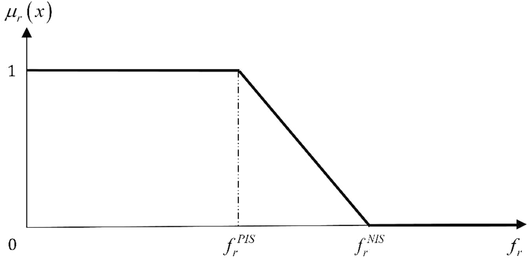
Step 2. As each objective function can be related to a fuzzy membership function (MF), therefore, the MFs of the objective functions are calculated by the following relationships (see also Fig. 3),
(43)
\[\begin{aligned}{}& {\mu _{1}}(x)=\left\{\begin{array}{l@{\hskip4.0pt}l}1\hspace{1em}& \text{if}\hspace{2.5pt}{f_{1}}\leqslant {f_{1}^{\mathit{PIS}}},\\ {} \frac{{f_{1}^{\mathit{NIS}}}-{f_{1}}}{{f_{1}^{\mathit{NIS}}}-{f_{1}^{\mathit{PIS}}}}\hspace{1em}& \text{if}\hspace{2.5pt}{f_{1}^{\mathit{PIS}}}\leqslant {f_{1}}\leqslant {f_{1}^{\mathit{NIS}}},\\ {} 0\hspace{1em}& \text{if}\hspace{2.5pt}{f_{1}}\geqslant {f_{1}^{\mathit{NIS}}},\end{array}\right.\end{aligned}\]
(44)
\[\begin{aligned}{}& {\mu _{2}}(x)=\left\{\begin{array}{l@{\hskip4.0pt}l}1\hspace{1em}& \text{if}\hspace{2.5pt}{f_{2}}\leqslant {f_{2}^{\mathit{PIS}}},\\ {} \frac{{f_{2}^{\mathit{NIS}}}-{f_{2}}}{{f_{2}^{\mathit{NIS}}}-{f_{2}^{\mathit{PIS}}}}\hspace{1em}& \text{if}\hspace{2.5pt}{f_{2}^{\mathit{PIS}}}\leqslant {f_{2}}\leqslant {f_{2}^{\mathit{NIS}}},\\ {} 0\hspace{1em}& \text{if}\hspace{2.5pt}{f_{2}}\geqslant {f_{2}^{\mathit{NIS}}},\end{array}\right.\end{aligned}\]
(45)
\[\begin{aligned}{}& {\mu _{3}}(x)=\left\{\begin{array}{l@{\hskip4.0pt}l}1\hspace{1em}& \text{if}\hspace{2.5pt}{f_{3}}\leqslant {f_{3}^{\mathit{PIS}}},\\ {} \frac{{f_{3}^{\mathit{NIS}}}-{f_{3}}}{{f_{3}^{\mathit{NIS}}}-{f_{3}^{\mathit{PIS}}}}\hspace{1em}& \text{if}\hspace{2.5pt}{f_{3}^{\mathit{PIS}}}\leqslant {f_{3}}\leqslant {f_{3}^{\mathit{NIS}}},\\ {} 0\hspace{1em}& \text{if}\hspace{2.5pt}{f_{3}}\geqslant {f_{3}^{\mathit{NIS}}},\end{array}\right.\end{aligned}\]
where ${\mu _{r}}(x)$ for $r\in \{1,2,\dots ,R\}$ (where $R=3$) is the linear MF of the objective function ${f_{r}}$.
info1219_g003.jpg
Fig. 3
Schematic representation of the fuzzy membership functions (Zimmermann, 1996).
Step 3 (Single-objective model step). Convert the multi-objective problem (24)–(36) to the following proposed single objective formulation.
(46)
\[\begin{aligned}{}& \max \frac{1}{R}{\sum \limits_{r=1}^{R}}{\theta _{r}}({\lambda _{r}}-{\lambda _{0}})\\ {} & \text{subject to}\\ {} & {\theta _{r}}{\lambda _{0}}+{\lambda _{r}}\leqslant {\mu _{r}}(x)\hspace{1em}\forall r\in \{1,2,\dots ,R\}\\ {} & {\lambda _{0}},{\lambda _{r}}\in [0,1]\hspace{1em}\forall r\in \{1,2,\dots ,R\}\\ {} & \text{Constraints (27)--(36)}.\end{aligned}\]
In the formulation (46), the positive value ${\theta _{r}}$ is the importance weight of r-th objective function with the condition of ${\textstyle\sum _{r=1}^{R}}{\theta _{r}}=1$. The continuous and non-negative variables ${\lambda _{0}}$ and ${\lambda _{r}}$ ($r\in \{1,2,\dots ,R\}$) are used to control the minimum satisfaction level of the objective functions as well as their compromise degrees.
Step 4. Solve the single-objective model (46) with a given set of values for weights of the objective functions (${\theta _{r}}$). If the obtained solution satisfies the decision maker, stop. Otherwise, do one of the following changes and repeat the steps 1 to 4 until a satisfactory solution is obtained.
  • • Increase the NIS value for maximization type objective functions,
  • • Decrease the PIS value for minimization type objective functions,
  • • Change the given set of values for weights of the objective functions (${\theta _{r}}$).

3.2 On the Single-Objective Model Step (Model (46)) of the Proposed Approach

As the most important step of any hybrid version of fuzzy programming approach is single-objective model phase, some advantages of single-objective model of the proposed approach of this study (formulation (46)), are detailed here:
  • • The optimization procedure of the single-objective model is done in one phase.
  • • Obtaining unique or efficient solution is guaranteed.
  • • The varying weights of the objective functions are eliminated.
  • • Membership function values are not used in the objective function.
  • • The goals are partially prioritized in the objective function and constraints. The weight of membership functions in the objective function depends on the number of objective functions of the main problem.
Of course, some of these advantages can reflect the differences of the proposed single-objective model of this study with those of the literature. The last three advantages are actually the difference of the proposed single-objective model with those of the literature.
The feasibility and efficiency of the formulation (46) is also detailed by Theorem 1.
Theorem 1.
Formulation (46) has a solution and its solution is efficient to the multi-objective problem (24)–(36).
Proof.
Let’s first define the following formulation which is a part of formulation (46).
(47)
\[\begin{aligned}{}& \max {\lambda _{0}}\\ {} & \text{subject to}\\ {} & {\lambda _{0}}\leqslant {\mu _{r}}(x)\hspace{1em}\forall r\in \{1,2,\dots ,R\}\\ {} & {\lambda _{0}}\in [0,1]\hspace{1em}\forall r\in \{1,2,\dots ,R\}\\ {} & \text{Constraints (27)--(36)}.\end{aligned}\]
Clearly, considering sign of constraints and type of objective function, problem (47) has an optimal solution (say, ${x^{0}}$). Now, considering ${\theta _{r}}$ values which are between zero and one, ${x^{0}}$ and ${\lambda _{r}}=0$ $(r\in \{1,2,\dots ,R\})$ together is a feasible solution to the problem (46). Therefore, the feasible region of the problem (46) is not empty.
The efficiency of the solution of model (46) is proved by a contradiction. Suppose that ${x^{\ast }}$ is an optimal solution of model (46) which is inefficient solution to the problem (24)–(36). Therefore, there should be an efficient solution like ${x^{\ast \ast }}$ to the problem (24)–(36) which is obtained by model (46) satisfying the conditions
  • i. ${f_{r}}({x^{\ast \ast }})\leqslant {f_{r}}({x^{\ast }})$ ($\forall r\in \{1,2,\dots ,R\}$) and $\exists i\in [0,1]:{f_{i}}({x^{\ast \ast }})<{f_{i}}({x^{\ast }})$,
  • ii. ${\mu _{r}}({x^{\ast \ast }})\geqslant {\mu _{r}}({x^{\ast }})$ ($\forall r\in \{1,2,\dots ,R\}$) and $\exists \hspace{0.1667em}i\in [0,1]:{\mu _{i}}({x^{\ast \ast }})>{\mu _{i}}({x^{\ast }})$.
So, to respect the minimum satisfaction level of the objectives of ${x^{\ast }}$ and ${x^{\ast \ast }}$, the condition ${\lambda _{0}^{\ast \ast }}\geqslant {\lambda _{0}^{\ast }}$ should be true. Now, considering the objective functions of these two solutions in formulation (46), the following inequality is obtained:
(48)
\[\begin{aligned}{}& \Bigg\{\frac{1}{R}{\sum \limits_{r=1}^{R}}{\theta _{r}}\big({\lambda _{r}^{\ast }}-{\lambda _{0}^{\ast }}\big)=\frac{1}{R}\Bigg({\sum \limits_{\substack{r=1\\ {} r\ne i}}^{R}}{\theta _{r}}\big({\lambda _{r}^{\ast }}-{\lambda _{0}^{\ast }}\big)+{\theta _{i}}\big({\lambda _{i}^{\ast }}-{\lambda _{0}^{\ast }}\big)\Bigg)\Bigg\}\\ {} & \hspace{1em}<\Bigg\{\frac{1}{R}{\sum \limits_{r=1}^{R}}{\theta _{r}}\big({\lambda _{r}^{\ast \ast }}-{\lambda _{0}^{\ast }}\big)=\frac{1}{R}\Bigg({\sum \limits_{\substack{r=1\\ {} r\ne i}}^{R}}{\theta _{r}}\big({\lambda _{r}^{\ast \ast }}-{\lambda _{0}^{\ast }}\big)+{\theta _{i}}\big({\lambda _{i}^{\ast \ast }}-{\lambda _{0}^{\ast }}\big)\Bigg)\Bigg\}.\end{aligned}\]
Therefore, ${x^{\ast }}$ is not an optimal solution of the problem (46) which is contradictory to the initial assumption for ${x^{\ast }}$ and the theorem is proved.  □

3.3 Comparison Metrics

In order to compare the performance of the proposed approach of this study to the other methods of the literature presented in the previous sub-section, the following distance measure is used (Alavidoost et al., 2016),
(49)
\[ {D_{p}}(\theta ,R)=\sqrt[1/p]{{\sum \limits_{r=1}^{R}}{\theta _{r}^{p}}{\big(1-{\mu _{r}}(x)\big)^{p}}}\hspace{1em}\forall p\geqslant 1\hspace{2.5pt}\text{and integer}.\]
Some well-known distance measures obtained from formula (49) are defined below.
Manhattan distance ($p=1$): This distance is actually the weighted sum of distance from goal which takes value of one here. The value of this distance has inverse relation with the value of MF as follows:
(50)
\[ {D_{1}}(\theta ,R)=1-{\sum \limits_{r=1}^{R}}{\theta _{r}}{\mu _{r}}(x).\]
Euclidean distance ($p=2$): This distance plays the same role as Manhattan distance. In addition, the quality of membership function values are evaluated. Meaning that closer MF values give less distance in the case of equal solutions.
(51)
\[ {D_{2}}(\theta ,R)=\sqrt{{\sum \limits_{r=1}^{R}}{\theta _{r}^{2}}{\big(1-{\mu _{r}}(x)\big)^{2}}}.\]
Tchebycheff distance ($p=\infty $): This is the shortest distance comparing to the above two distances. When this distance (also other distances with $p>1$) is calculated, more penalty is given to the smaller MF values. Therefore, the solutions having close MFs will get less distance value when this distance is considered.
(52)
\[ {D_{\infty }}(\theta ,R)=\underset{R}{\max }\big\{{\theta _{r}}\big(1-{\mu _{r}}(x)\big)\big\}.\]

4 Computational Experiments

info1219_g004.jpg
Fig. 4
The precedence graph of test problem 1.
The proposed multi-objective formulation (24)–(36) and its proposed solution approach are computationally experimented in this section using two test problems. The experiments are done for two purposes. First an analysis is done for linearization procedure of entropy-based objective function, then wide experiments are done to measure the performance of the proposed solution approach. For this aim the mathematical models are solved using GAMS 23.5 solver. The experiments are reported in the following sub-sections.

4.1 Test Problems

Two test problems are considered to evaluate the performance of the solution approach of this study. These are taken from the literature of assembly line balancing problem and are modified by adding some required data for the new parameters which are new in this study.
Test problem 1 (Jackson, 1956) consists of 11 tasks with the precedence graph of Fig. 4. The task times (in minutes) are shown above of the nodes. The worker time-dependent wage for the tasks are integer random values (cents of dollar) uniformly distributed on the interval $[1,9]$. There are four equipment to be used in the line for performing the tasks with purchasing costs of $5000, $8000, $6000, and $11000. Depending on technical process needed for each task, some or all of them are needed. Cycle time of 15 minutes and number of stations 5 are also considered.
Test problem 2 (Mitchell, 1957; Tonge, 1960) consists of 21 tasks with the precedence graph of Fig. 5. The task times (in minutes) are shown above of the nodes. The worker time-dependent wage for the tasks are integer random values (cents of dollar) uniformly distributed on the interval $[1,9]$. There are four equipment to be used in the line for performing the tasks with purchasing costs of $5600, $6800, $10000, and $4200. Depending on technical process needed for each task, some or all of them are needed. Cycle time of 20 minutes and number of stations 6 are also considered.

4.2 Sensitivity Analysis on the Linearized Entropy Objective Function

info1219_g005.jpg
Fig. 5
The precedence graph of test problem 2.
In this section the performance of linearization technique used for entropy objective function (5)–(6) is studied. In linearization technique the entropy function was divided to some linear segments. So, the model (20)–(23) was introduced as its linearized form. The formulation (20)–(23) is sensitive to two factors (i) number of segments, (ii) length of each segment. To have a good approximation for entropy objective function (5)–(6) these factors should be tuned. In this section we try to tune the first factor by the assumption that the segments have equal lengths. Therefore, the following steps are done to measure the performance of the linearization technique.
  • 1. Test problem 2 is selected for this aim.
  • 2. A feasible solution is generated manually to respect the constraints (12)–(14).
  • 3. The solution is evaluated by model (5)–(6) to obtain its entropy objective function value (${f_{\mathit{entropy}}}$).
  • 4. The solution is evaluated by model (20)–(23) to obtain its linearized objective function value (${f_{L\text{-}\mathit{entropy}}}$). In this step the number of segments and their lengths is given to the model. Therefore, the tuning is actually done in this step. We vary the number of segments to study the impact of this factor on the linearization technique.
The number of segments and their associated lengths are shown in Table 2. Therefore, each experiment is specified by a number of segments and their equal lengths which is obtained from dividing one by the number of segments ($\frac{1}{P}$). The generated feasible solution is evaluated by models (5)–(6) and (20)–(23) separately. The results are shown by Table 2.
Table 2
The results obtained for parameter tuning of the linearization technique.
Experiment Number of segments $(P)$ Equal length of the segments (${\alpha _{pk}}$) ${f_{L\text{-}\mathit{entropy}}}$ ${f_{\mathit{entropy}}}$
1 5 0.200 −1.609 −1.778
2 10 0.100 −1.748
3 16 0.062 −1.768
4 20 0.050 −1.770
5 40 0.025 −1.776
6 70 0.014 −1.777
7 100 0.010 −1.778
info1219_g006.jpg
Fig. 6
Schematic representation of the performances of the entropy objective function and its linearized form.
According to the results of Table 2, higher number of segments results in a better linear approximation of the entropy objective function (5)–(6). Notably, when the number of segments is equal to 100, in the case of this study, although the number of constraints of the main model is increased, the entropy objective function and its linearized form give the same objective value. The performances are also shown in the graph of Fig. 6.

4.3 Final Computational Experiments

To measure the ability of the proposed approach the model (24)–(36) was solved for the test problems of subsection 4.1. To make comparisons with the methods of literature, these test problems were also solved by the methods of literature like SO, TH, DY, and ABS. To perform these runs, the following assumptions were considered:
  • • The number of segments $(P)$ in the linearized entropy objective function was set to be 20.
  • • To make a more detailed performance analysis, five combination of values for the weights (${\theta _{r}}$) were applied as depicted in Table 3.
  • • In some of the methods, another weight (say λ) is needed. In the experiments of the literature 0.4 was used as its best value. In this study also the same value is used for λ.
    Table 3
    Different combinations of weights used to run the proposed method and the methods of literature.
    Combination ${\theta _{1}}$ ${\theta _{2}}$ ${\theta _{3}}$
    C 1 0.20 0.30 0.50
    c 2 0.30 0.40 0.30
    C 3 0.33 0.33 0.34
    C 4 0.40 0.30 0.30
    C 5 0.50 0.25 0.25
    Table 4
    The positive and negative ideal solutions obtained for each objective function.
    Objective function Ideal solution Test problem
    Test problem 1 Test problem 2
    ${f_{1}}$ ${f_{1}^{\mathit{PIS}}}$ −1.544 −1.776
    ${f_{1}^{\mathit{NIS}}}$ 0.883 0.909
    ${f_{2}}$ ${f_{2}^{\mathit{PIS}}}$ 88000 144000
    ${f_{2}^{\mathit{NIS}}}$ 150000 159600
    ${f_{3}}$ ${f_{3}^{\mathit{PIS}}}$ 330 880
    ${f_{3}^{\mathit{NIS}}}$ 675 1080
  • • In some of the methods, a coefficient (say δ) is needed. In the experiments of the literature 0.01 was used as its best value. In this study also the same value is used for δ.
Table 5
The result obtained for test problem 1.
Weights Method ${\mu _{1}}(x)$ ${\mu _{2}}(x)$ ${\mu _{3}}(x)$ ${D_{1}}(\theta ,R)$ ${D_{2}}(\theta ,R)$ ${D_{\infty }}(\theta ,R)$
C1 ABS 0.867 0.581 1 0.152 0.129 0.126
DY 0.792 0.661 1 0.143 0.11 0.102
TH 0.904 1 0.783 0.128 0.11 0.109
SO 0.926 0.871 0.87 0.119 0.077 0.065
The proposed approach 0.926 0.871 0.87 0.119 0.077 0.065
C2 ABS 0.904 1 0.783 0.094 0.071 0.065
DY 0.816 1 0.783 0.12 0.085 0.065
TH 0.913 0.919 0.826 0.11 0.067 0.052
SO 0.904 1 0.783 0.094 0.071 0.065
The proposed approach 0.904 1 0.783 0.094 0.071 0.065
C3 ABS 0.926 0.871 0.87 0.111 0.066 0.044
DY 0.844 0.871 0.87 0.138 0.08 0.051
TH 0.913 0.919 0.826 0.114 0.071 0.059
SO 0.904 1 0.783 0.106 0.08 0.074
The proposed approach 0.904 1 0.783 0.106 0.08 0.074
C4 ABS 1 0.742 0.696 0.169 0.12 0.091
DY 0.926 0.71 0.87 0.156 0.1 0.087
TH 0.904 1 0.783 0.104 0.076 0.065
SO 0.904 1 0.783 0.104 0.076 0.065
The proposed approach 0.904 1 0.783 0.104 0.076 0.065
C5 ABS 0.929 0.468 0.609 0.266 0.169 0.133
DY 0.993 0.694 0.696 0.156 0.108 0.077
TH 0.904 1 0.783 0.103 0.073 0.054
SO 0.904 1 0.783 0.103 0.073 0.054
The proposed approach 0.926 0.871 0.87 0.102 0.059 0.037
The test problems were solved by sub-models (37)–(42) to obtain the positive ideal solution (POS) and negative ideal solution (NIS) of each objective function individually. These are the result of Step 2 of the proposed approach which is also a common step for the methods of literature. The results are presented by Table 4.
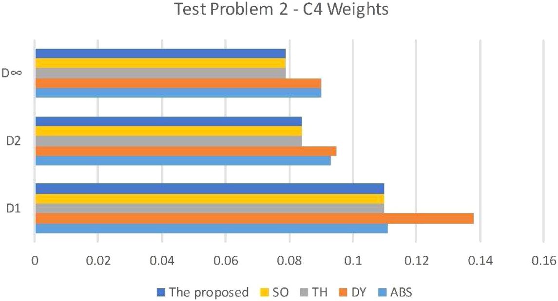
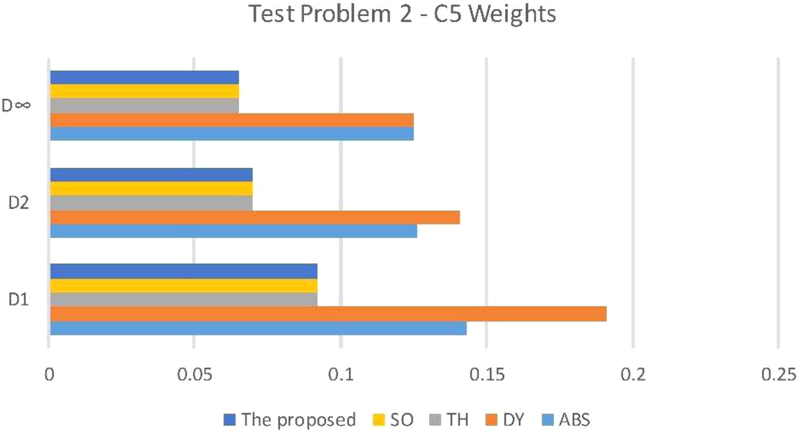
Finally, applying the above-mentioned test problems, the model (24)–(36) was solved by the proposed approach of this study (Step 3) and the methods of literature. In all the experiments the above-mentioned assumptions and the result of Table 4 were considered. The results are shown by Table 5 and Table 6 and also the charts provided in Figs. 7–16.
info1219_g007.jpg
Fig. 7
Chart of the performance of the proposed and employed approaches for test problem 1 with weight combination C1.
Table 6
The result obtained for test problem 2.
Weights Method ${\mu _{1}}(x)$ ${\mu _{2}}(x)$ ${\mu _{3}}(x)$ ${D_{1}}(\theta ,R)$ ${D_{2}}(\theta ,R)$ ${D_{\infty }}(\theta ,R)$
C1 ABS 0.997 0.738 0.9 0.129 0.093 0.079
DY 0.911 0.738 0.9 0.146 0.096 0.079
TH 0.997 0.738 0.9 0.129 0.093 0.079
SO 0.997 0.738 0.9 0.129 0.093 0.079
The proposed approach 0.997 0.738 0.9 0.129 0.093 0.079
C2 ABS 1 0.929 0.7 0.119 0.094 0.09
DY 0.913 0.929 0.7 0.145 0.099 0.09
TH 0.997 0.738 0.9 0.136 0.109 0.105
SO 1 0.929 0.7 0.119 0.094 0.09
The proposed approach 1 0.929 0.7 0.119 0.094 0.09
C3 ABS 0.997 0.738 0.9 0.122 0.093 0.086
DY 0.911 0.738 0.9 0.15 0.097 0.086
TH 0.997 0.738 0.9 0.122 0.093 0.086
SO 0.997 0.738 0.9 0.122 0.093 0.086
The proposed approach 0.997 0.738 0.9 0.122 0.093 0.086
C4 ABS 1 0.929 0.7 0.111 0.093 0.09
DY 0.933 0.929 0.7 0.138 0.095 0.09
TH 0.997 0.738 0.9 0.11 0.084 0.079
SO 0.997 0.738 0.9 0.11 0.084 0.079
The proposed approach 0.997 0.738 0.9 0.11 0.084 0.079
C5 ABS 1 0.929 0.5 0.143 0.126 0.125
DY 0.999 0.738 0.5 0.191 0.141 0.125
TH 0.997 0.738 0.9 0.092 0.07 0.065
SO 0.997 0.738 0.9 0.092 0.07 0.065
The proposed approach 0.997 0.738 0.9 0.092 0.07 0.065
info1219_g008.jpg
Fig. 8
Chart of the performance of the proposed and employed approaches for test problem 1 with weight combination C2.
According to the obtained results for test problem 1, the proposed approach is better than the other approaches of the literature in most of the weight combinations. As can be concluded from Table 5, in C1 combination of weights, in the case of all distance metrics both SO and the proposed approaches have the same performance which is better than the other approaches. When the weights are changed to C2, considering ${D_{1}}$ measure, the methods ABS, SO, and the proposed approach perform as the best, but in the case of ${D_{2}}$ and ${D_{\infty }}$ distances, TH approach has the best performance among all. In the case of C3 weights, considering ${D_{1}}$ measure, the methods SO and the proposed approach perform as the best, but in the case of ${D_{2}}$ and ${D_{\infty }}$ distances, ABS approach has the best performance among all. Using C4 combination of weights, in the case of all distance metrics, the methods TH, SO, and the proposed approach have the same performance which is better than that of the other approaches. Finally, applying the last combination of weights C5, the proposed method of this study outperforms other approaches uniquely.
info1219_g009.jpg
Fig. 9
Chart of the performance of the proposed and employed approaches for test problem 1 with weight combination C3.
info1219_g010.jpg
Fig. 10
Chart of the performance of the proposed and employed approaches for test problem 1 with weight combination C4.
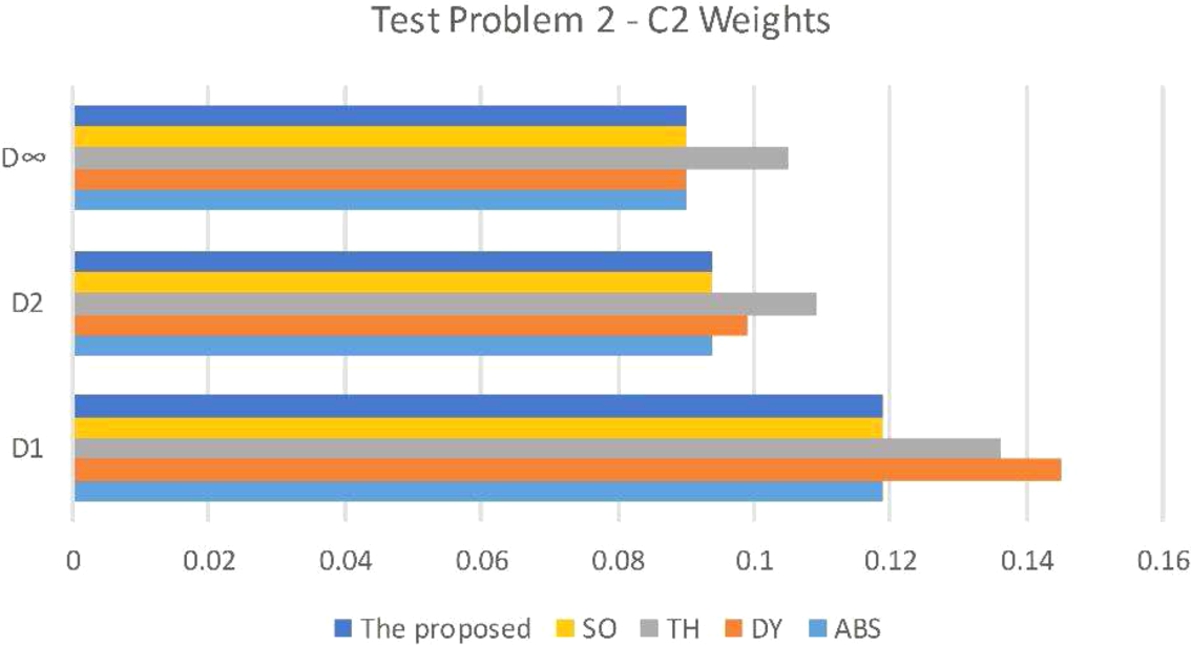
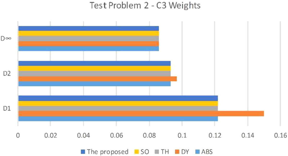
As an analysis to the obtained results for test problem 2, the proposed approach is among the best performed approaches in all the weight combinations. As can be concluded from Table 6, in C1 combination of weights, in the case of all distance metrics the methods ABS, TH, SO, and the proposed approach perform as the best. When the weights are changed to C2, in the case of all distance metrics the methods ABS, SO, and the proposed approach perform as the best. In the case of C3 weights, in the case of all distance metrics the methods ABS, TH, SO, and the proposed approach perform as the best. Using C4 combination of weights, in the case of all distance metrics, the methods TH, SO, and the proposed approaches have the same performance which is better than that of the other approaches. Finally, applying the last combination of weights C5, in the case of all distance metrics the methods TH, SO, and the proposed approach perform as the best.
info1219_g011.jpg
Fig. 11
Chart of the performance of the proposed and employed approaches for test problem 1 with weight combination C5.
info1219_g012.jpg
Fig. 12
Chart of the performance of the proposed and employed approaches for test problem 2 with weight combination C1.

5 Concluding Remarks

A typical assembly line balancing problem with different scale objective functions was studied in this paper. An entropy function was used as an objective function in order to balance the work load of the stations of assembly line plus two more objective functions like equipment purchasing cost and worker time-dependent wage. The most important limitations of this problem were its non-linearity and its multi-objective nature. The non-linearity of the entropy-based objective function was approximated as a linear function using the bounded variable method of linear programming. A new hybrid fuzzy programming approach was developed to solve the proposed multi-objective formulation. In order to compare the efficient solutions of the problem, three distance metrics were used. The required computational experiments were performed by the proposed hybrid fuzzy programming approach and some other approaches of the literature on some test problems. According to the obtained results and using the distance metrics, the proposed solution approach performs either the same or better than the multi-objective solution approaches of the literature like ABD, DY, TH, and SO.
info1219_g013.jpg
Fig. 13
Chart of the performance of the proposed and employed approaches for test problem 2 with weight combination C2.
info1219_g014.jpg
Fig. 14
Chart of the performance of the proposed and employed approaches for test problem 2 with weight combination C3.
info1219_g015.jpg
Fig. 15
Chart of the performance of the proposed and employed approaches for test problem 2 with weight combination C4.
info1219_g016.jpg
Fig. 16
Chart of the performance of the proposed and employed approaches for test problem 2 with weight combination C5.

Acknowledgment.

We are grateful to the editors and anonymous reviewers of the journal for their helpful and constructive comments that helped us to improve the quality of the paper.

References

 
Alavidoost, M.H., Tarimoradi, M., Fazel Zarandi, M.H. (2015). Fuzzy adaptive genetic algorithm for multi-objective assembly line balancing problems. Applied Soft Computing, 34, 655–677.
 
Alavidoost, M.H., Babazadeh, H., Sayyari, S.T. (2016). An interactive fuzzy programming approach for bi-objective straight and U-shaped assembly line balancing problem. Applied Soft Computing, 40, 221–235.
 
Amen, M. (2001). Heuristic methods for cost-oriented assembly line balancing: A comparison on solution quality and computing time. International Journal of Production Economics, 69(3), 255–264.
 
Amen, M. (2006). Cost-oriented assembly line balancing: Model formulations, solution difficulty, upper and lower bounds. European Journal of Operational Research, 168(3), 747–770.
 
Battini, D., Delorme, X., Dolgui, A., Sgarbossa, S. (2015). Assembly line balancing with ergonomics paradigms: two alternative methods. IFAC-PapersOnLine, 48(3), 586–591.
 
Baybars, I. (1986). A survey of exact algorithms for the simple assembly line balancing problem. Management Science, 32, 909–932.
 
Borba, L., Ritt, M., Miralles, C. (2018). Exact and heuristic methods for solving the Robotic Assembly Line Balancing Problem. European Journal of Operational Research, 270(1), 146–156.
 
Buyukozkan, K., Kucukkoc, I., Satoglu, S.I., Zhang, D.Z. (2016). Lexicographic bottleneck mixed-model assembly line balancing problem: Artificial bee colony and tabu search approaches with optimised parameters. Expert Systems with Applications, 50, 151–166.
 
Dantzig, G.B. (1963). Linear Programming and Extensions. Princeton University Press, Princeton, United States.
 
Demirli, K., Yimer, A.D. (2008). Fuzzy scheduling of a build-to-order supply chain. International Journal of Production Research, 46, 3931–3958.
 
Fattahi, A., Turkay, M. (2015). On the MILP model for the U-shaped assembly line balancing problems. European Journal of Operational Research, 242(1), 343–346.
 
Hajipour, V., Fattahi, P., Tavana, M., Di Caprio, D. (2016). Multi-objective multi-layer congested facility location-allocation problem optimization with Pareto-based meta-heuristics. Applied Mathematical Modelling, 40(7–8), 4948–4969.
 
Hazır, Ö., Dolgui, A. (2015). A decomposition based solution algorithm for U-type assembly line balancing with interval data. Computers & Operations Research, 59, 126–131.
 
Jablonsky, J. (2007). Measuring the efficiency of production units by AHP models. Mathematical and Computer Modelling, 46(7–8), 1091–1098.
 
Jablonsky, J. (2014). MS Excel based software support tools for decision problems with multiple criteria. Procedia Economics and Finance, 12, 251–258.
 
Jackson, J.R. (1956). A computing procedure for a line balancing problem. Management Science, 2, 261–271.
 
Keshavarz Ghorabaee, M., Amiri, M., Turskis, Z. (2017). A new approach for solving bi-objective redundancy allocation problem using DOE, simulation and ε-constraint method. Informatica, 28(1), 79–104.
 
Kovács, G., Marian, M. (2002). Viability results in control of one-dimensional discrete time dynamical systems defined by a multi-function. Pure Mathematics and Applications, 13(1–2), 185–195.
 
Kucukkoc, I., Zhang, D.Z. (2014). Mathematical model and agent based solution approach for the simultaneous balancing and sequencing of mixed-model parallel two-sided assembly lines. International Journal of Production Economics, 158, 314–333.
 
Kucukkoc, I., Zhang, D.Z. (2016). Mixed-model parallel two-sided assembly line balancing problem: a flexible agent-based ant colony optimization approach. Computers & Industrial Engineering, 97, 58–72.
 
Lea, D., Gub, X. (2016). Variable neighborhood search for the second type of two-sided assembly line balancing problem. Computers & Operations Research, 72, 183–188.
 
Mardani-Fard, H.A., Hadi-Vencheh, A., Mahmoodirad, A., Niroomand, S. (2018). An effective hybrid goal programming approach for multi-objective straight assembly line balancing problem with stochastic parameters. Operational Research. doi:10.1007/s12351-018-0428-8.
 
Mitchell, J. (1957). A Computational Procedure for Balancing Zoned Assembly Lines. Research Report 6-94801-1-R3, Westinghouse Research Laboratories, Pittsburgh.
 
Ogan, D., Azizoglu, M. (2015). A branch and bound method for the line balancing problem in U-shaped assembly lines with equipment requirements. Journal of Manufacturing Systems, 36, 46–54.
 
Ojha, A., Das, N., Mondal, S., Maiti, M. (2009). An entropy based solid transportation problem for general fuzzy costs and time with fuzzy equality. Mathematical and Computer Modelling, 50, 166–178.
 
Pereira, J., Álvarez-Miranda, E. (2018). An exact approach for the robust assembly line balancing problem. Omega, 78, 85–98.
 
Ramezanian, R., Ezzatpanah, A. (2015). Modeling and solving multi-objective mixed-model assembly line balancing and worker assignment problem. Computers & Industrial Engineering, 87, 74–80.
 
Salehi, M., Maleki, H.R., Niroomand, S. (2018). A multi-objective assembly line balancing problem with worker’s skill and qualification considerations in fuzzy environment. Applied Intelligence, 48(8), 2137–2156.
 
Samouei, P., Fattahi, P., Ashayeri, J., Ghazinoory, S. (2016). Bottleneck easing-based assignment of work and product mixture determination: fuzzy assembly line balancing approach. Applied Mathematical Modelling, 40(7–8), 4323–4340.
 
Selim, H., Ozkarahan, I. (2008). A supply chain distribution network design model: an interactive fuzzy goal programming-based solution approach. International Journal of Advanced Manufacturing Technology, 36, 401–418.
 
Sepahi, A., Jalali Naini, S.J. (2016). Two-sided assembly line balancing problem with parallel performance capacity. Applied Mathematical Modelling, 40(13–14), 6280–6292.
 
Shannon, C.E. (1948). A mathematical theory of communication. Bell System Technical Journal, 27(3), 379–423.
 
Sun, H., Chen, R., Qin, Y., Wang, S. (2017). Holo-entropy based categorical data hierarchical clustering. Informatica, 28(2), 303–328.
 
Tavana, M., Abtahi, A.R., Khalili-Damghani, K. (2014a). A new multi-objective multi-mode model for solving preemptive time-cost-quality trade-off project scheduling problems. Expert Systems with Applications, 41(4), 1830–1846.
 
Tavana, M., Fazlollahtabar, H., Hassanzade, R. (2014b). A bi-objective stochastic programming model for optimising automated material handling systems with reliability considerations. International Journal of Production Research, 52(19), 5597–5610.
 
Tavana, M., Li, Z., Mobin, M., Komaki, G.M., Teymourian, E. (2016). Multi-objective control chart design. optimization using NSGA-III and MOPSO enhanced with DEA and TOPSIS. Expert Systems with Applications, 50, 17–39.
 
Tonge, F.M. (1960). Summary of a heuristic line balancing procedure. Management Science, 7, 21–39.
 
Torabi, S.A., Hassini, E. (2008). An interactive possibilistic programming approach for multiple objective supply chain master planning. Fuzzy Sets and Systems, 159, 193–214.
 
Tuncel, G., Aydin, D. (2014). Two-sided assembly line balancing using teaching–learning based optimization algorithm. Computers & Industrial Engineering, 74, 291–299.
 
Yang, C., Gao, J. (2016). Balancing mixed-model assembly lines using adjacent cross-training in a demand variation environment. Computers & Operations Research, 65, 139–148.
 
Yuguang, Z., Bo, A., Yong, Z. (2016). A PSO algorithm for multi-objective hull assembly line balancing using the stratified optimization strategy. Computers & Industrial Engineering, 98, 53–62.
 
Zacharia, Th. Nearchou A. C, P. (2016). A population-based algorithm for the bi-objective assembly line worker assignment and balancing problem. Engineering Applications of Artificial Intelligence, 49, 1–9.
 
Zimmermann, H.J. (1996). Fuzzy Set Theory and Its Applications. Kluwer-Nijhoff, Boston, United States.
 
Zeng, S., Gonzalez, J., Lobato, C. (2015). The effect of organizational learning and Web 2.0 on innovation. Management Decision, 53(9), 2060–2072.
 
Zeng, S., Palacios-Marques, D., Zhu, F. (2016). A new model for interactive group decision making with intuitionistic fuzzy preference relations. Informatica, 27(4), 911–928.

Biographies

Mahmoodirad Ali

A. Mahmoodirad is an assistant professor of applied mathematics (operation research) in Masjed-Soleiman Branch of Islamic Azad University in Iran. His research interests include fuzzy mathematical programming, supply chain management, transportation problems and decomposition methods.

Heydari Ahmad

A. Heydari is a faculty member at Firouzabad Institute of Higher Education in Iran. He received his master’s degree in mathematics from Shahid Beheshti University (in Iran).

Niroomand Sadegh
sadegh.niroomand@yahoo.com

S. Niroomand is an assistant professor of industrial engineering in Firouzabad Institute of Higher Education in Iran. He received his PhD degree in industrial engineering from Eastern Mediterranean University (in Turkey), in 2013. His research interests are operations research, fuzzy theory, and exact and meta-heuristic solution approaches.


Reading mode PDF XML

Table of contents
  • 1 Introduction
  • 2 Multi-Objective Entropy-Based Assembly Line Balancing Problem
  • 3 Solution Approaches
  • 4 Computational Experiments
  • 5 Concluding Remarks
  • Acknowledgment.
  • References
  • Biographies

Copyright
© 2019 Vilnius University
by logo by logo
Open access article under the CC BY license.

Keywords
assembly line balancing problem entropy function bounded variable linearization method fuzzy programming approach

Metrics
since January 2020
1146

Article info
views

674

Full article
views

605

PDF
downloads

220

XML
downloads

Export citation

Copy and paste formatted citation
Placeholder

Download citation in file


Share


RSS

  • Figures
    16
  • Tables
    6
  • Theorems
    1
info1219_g001.jpg
Fig. 1
A graphical illustration of input (a) and output (b and c) for a simple assembly line balancing problem.
info1219_g002.jpg
Fig. 2
Schematic representation of the bounded variable approximation method.
info1219_g003.jpg
Fig. 3
Schematic representation of the fuzzy membership functions (Zimmermann, 1996).
info1219_g004.jpg
Fig. 4
The precedence graph of test problem 1.
info1219_g005.jpg
Fig. 5
The precedence graph of test problem 2.
info1219_g006.jpg
Fig. 6
Schematic representation of the performances of the entropy objective function and its linearized form.
info1219_g007.jpg
Fig. 7
Chart of the performance of the proposed and employed approaches for test problem 1 with weight combination C1.
info1219_g008.jpg
Fig. 8
Chart of the performance of the proposed and employed approaches for test problem 1 with weight combination C2.
info1219_g009.jpg
Fig. 9
Chart of the performance of the proposed and employed approaches for test problem 1 with weight combination C3.
info1219_g010.jpg
Fig. 10
Chart of the performance of the proposed and employed approaches for test problem 1 with weight combination C4.
info1219_g011.jpg
Fig. 11
Chart of the performance of the proposed and employed approaches for test problem 1 with weight combination C5.
info1219_g012.jpg
Fig. 12
Chart of the performance of the proposed and employed approaches for test problem 2 with weight combination C1.
info1219_g013.jpg
Fig. 13
Chart of the performance of the proposed and employed approaches for test problem 2 with weight combination C2.
info1219_g014.jpg
Fig. 14
Chart of the performance of the proposed and employed approaches for test problem 2 with weight combination C3.
info1219_g015.jpg
Fig. 15
Chart of the performance of the proposed and employed approaches for test problem 2 with weight combination C4.
info1219_g016.jpg
Fig. 16
Chart of the performance of the proposed and employed approaches for test problem 2 with weight combination C5.
Table 1
Notationsused for mathematical formulations.
Table 2
The results obtained for parameter tuning of the linearization technique.
Table 3
Different combinations of weights used to run the proposed method and the methods of literature.
Table 4
The positive and negative ideal solutions obtained for each objective function.
Table 5
The result obtained for test problem 1.
Table 6
The result obtained for test problem 2.
Theorem 1.
info1219_g001.jpg
Fig. 1
A graphical illustration of input (a) and output (b and c) for a simple assembly line balancing problem.
info1219_g002.jpg
Fig. 2
Schematic representation of the bounded variable approximation method.
info1219_g003.jpg
Fig. 3
Schematic representation of the fuzzy membership functions (Zimmermann, 1996).
info1219_g004.jpg
Fig. 4
The precedence graph of test problem 1.
info1219_g005.jpg
Fig. 5
The precedence graph of test problem 2.
info1219_g006.jpg
Fig. 6
Schematic representation of the performances of the entropy objective function and its linearized form.
info1219_g007.jpg
Fig. 7
Chart of the performance of the proposed and employed approaches for test problem 1 with weight combination C1.
info1219_g008.jpg
Fig. 8
Chart of the performance of the proposed and employed approaches for test problem 1 with weight combination C2.
info1219_g009.jpg
Fig. 9
Chart of the performance of the proposed and employed approaches for test problem 1 with weight combination C3.
info1219_g010.jpg
Fig. 10
Chart of the performance of the proposed and employed approaches for test problem 1 with weight combination C4.
info1219_g011.jpg
Fig. 11
Chart of the performance of the proposed and employed approaches for test problem 1 with weight combination C5.
info1219_g012.jpg
Fig. 12
Chart of the performance of the proposed and employed approaches for test problem 2 with weight combination C1.
info1219_g013.jpg
Fig. 13
Chart of the performance of the proposed and employed approaches for test problem 2 with weight combination C2.
info1219_g014.jpg
Fig. 14
Chart of the performance of the proposed and employed approaches for test problem 2 with weight combination C3.
info1219_g015.jpg
Fig. 15
Chart of the performance of the proposed and employed approaches for test problem 2 with weight combination C4.
info1219_g016.jpg
Fig. 16
Chart of the performance of the proposed and employed approaches for test problem 2 with weight combination C5.
Table 1
Notationsused for mathematical formulations.
Notation Type Definition
$i(j)(I)$ Index/parameter index used for task (index used for task) (the number of tasks)
$k(r)(K)$ Index/parameter index used for station (index used for station) (the number of stations)
${t_{i}}$ Parameter processing time of task i
${\mathit{PR}_{i}}$ Parameter predecessor set of task i
${\mathit{SC}_{i}}$ Parameter successor set of task i
$\mathrm{CT}$ Variable cycle time
${X_{ik}}$ Variable 1, if task i is assigned to station k; 0, otherwise
Table 2
The results obtained for parameter tuning of the linearization technique.
Experiment Number of segments $(P)$ Equal length of the segments (${\alpha _{pk}}$) ${f_{L\text{-}\mathit{entropy}}}$ ${f_{\mathit{entropy}}}$
1 5 0.200 −1.609 −1.778
2 10 0.100 −1.748
3 16 0.062 −1.768
4 20 0.050 −1.770
5 40 0.025 −1.776
6 70 0.014 −1.777
7 100 0.010 −1.778
Table 3
Different combinations of weights used to run the proposed method and the methods of literature.
Combination ${\theta _{1}}$ ${\theta _{2}}$ ${\theta _{3}}$
C 1 0.20 0.30 0.50
c 2 0.30 0.40 0.30
C 3 0.33 0.33 0.34
C 4 0.40 0.30 0.30
C 5 0.50 0.25 0.25
Table 4
The positive and negative ideal solutions obtained for each objective function.
Objective function Ideal solution Test problem
Test problem 1 Test problem 2
${f_{1}}$ ${f_{1}^{\mathit{PIS}}}$ −1.544 −1.776
${f_{1}^{\mathit{NIS}}}$ 0.883 0.909
${f_{2}}$ ${f_{2}^{\mathit{PIS}}}$ 88000 144000
${f_{2}^{\mathit{NIS}}}$ 150000 159600
${f_{3}}$ ${f_{3}^{\mathit{PIS}}}$ 330 880
${f_{3}^{\mathit{NIS}}}$ 675 1080
Table 5
The result obtained for test problem 1.
Weights Method ${\mu _{1}}(x)$ ${\mu _{2}}(x)$ ${\mu _{3}}(x)$ ${D_{1}}(\theta ,R)$ ${D_{2}}(\theta ,R)$ ${D_{\infty }}(\theta ,R)$
C1 ABS 0.867 0.581 1 0.152 0.129 0.126
DY 0.792 0.661 1 0.143 0.11 0.102
TH 0.904 1 0.783 0.128 0.11 0.109
SO 0.926 0.871 0.87 0.119 0.077 0.065
The proposed approach 0.926 0.871 0.87 0.119 0.077 0.065
C2 ABS 0.904 1 0.783 0.094 0.071 0.065
DY 0.816 1 0.783 0.12 0.085 0.065
TH 0.913 0.919 0.826 0.11 0.067 0.052
SO 0.904 1 0.783 0.094 0.071 0.065
The proposed approach 0.904 1 0.783 0.094 0.071 0.065
C3 ABS 0.926 0.871 0.87 0.111 0.066 0.044
DY 0.844 0.871 0.87 0.138 0.08 0.051
TH 0.913 0.919 0.826 0.114 0.071 0.059
SO 0.904 1 0.783 0.106 0.08 0.074
The proposed approach 0.904 1 0.783 0.106 0.08 0.074
C4 ABS 1 0.742 0.696 0.169 0.12 0.091
DY 0.926 0.71 0.87 0.156 0.1 0.087
TH 0.904 1 0.783 0.104 0.076 0.065
SO 0.904 1 0.783 0.104 0.076 0.065
The proposed approach 0.904 1 0.783 0.104 0.076 0.065
C5 ABS 0.929 0.468 0.609 0.266 0.169 0.133
DY 0.993 0.694 0.696 0.156 0.108 0.077
TH 0.904 1 0.783 0.103 0.073 0.054
SO 0.904 1 0.783 0.103 0.073 0.054
The proposed approach 0.926 0.871 0.87 0.102 0.059 0.037
Table 6
The result obtained for test problem 2.
Weights Method ${\mu _{1}}(x)$ ${\mu _{2}}(x)$ ${\mu _{3}}(x)$ ${D_{1}}(\theta ,R)$ ${D_{2}}(\theta ,R)$ ${D_{\infty }}(\theta ,R)$
C1 ABS 0.997 0.738 0.9 0.129 0.093 0.079
DY 0.911 0.738 0.9 0.146 0.096 0.079
TH 0.997 0.738 0.9 0.129 0.093 0.079
SO 0.997 0.738 0.9 0.129 0.093 0.079
The proposed approach 0.997 0.738 0.9 0.129 0.093 0.079
C2 ABS 1 0.929 0.7 0.119 0.094 0.09
DY 0.913 0.929 0.7 0.145 0.099 0.09
TH 0.997 0.738 0.9 0.136 0.109 0.105
SO 1 0.929 0.7 0.119 0.094 0.09
The proposed approach 1 0.929 0.7 0.119 0.094 0.09
C3 ABS 0.997 0.738 0.9 0.122 0.093 0.086
DY 0.911 0.738 0.9 0.15 0.097 0.086
TH 0.997 0.738 0.9 0.122 0.093 0.086
SO 0.997 0.738 0.9 0.122 0.093 0.086
The proposed approach 0.997 0.738 0.9 0.122 0.093 0.086
C4 ABS 1 0.929 0.7 0.111 0.093 0.09
DY 0.933 0.929 0.7 0.138 0.095 0.09
TH 0.997 0.738 0.9 0.11 0.084 0.079
SO 0.997 0.738 0.9 0.11 0.084 0.079
The proposed approach 0.997 0.738 0.9 0.11 0.084 0.079
C5 ABS 1 0.929 0.5 0.143 0.126 0.125
DY 0.999 0.738 0.5 0.191 0.141 0.125
TH 0.997 0.738 0.9 0.092 0.07 0.065
SO 0.997 0.738 0.9 0.092 0.07 0.065
The proposed approach 0.997 0.738 0.9 0.092 0.07 0.065
Theorem 1.
Formulation (46) has a solution and its solution is efficient to the multi-objective problem (24)–(36).

INFORMATICA

  • Online ISSN: 1822-8844
  • Print ISSN: 0868-4952
  • Copyright © 2023 Vilnius University

About

  • About journal

For contributors

  • OA Policy
  • Submit your article
  • Instructions for Referees
    •  

    •  

Contact us

  • Institute of Data Science and Digital Technologies
  • Vilnius University

    Akademijos St. 4

    08412 Vilnius, Lithuania

    Phone: (+370 5) 2109 338

    E-mail: informatica@mii.vu.lt

    https://informatica.vu.lt/journal/INFORMATICA
Powered by PubliMill  •  Privacy policy