1 Introduction
The efficient market hypothesis states that financial tools such as stock prices or exchange rates move randomly. This implies that future prices are unpredictable. However, the amount of researches in forecasting financial markets is growing rapidly. Forecasting models combine different forecasting methods: time series forecasting, behavioural forecasting, expert evaluation methods and others. Different approaches to solving a problem are combined in one model with the aim of helping make the right solution at the right time. Bilson (
1981) presented a ‘speculative hypothesis’ that forward prices are the best unbiased forecast of future spot prices. Fama (
1984) associated a negative correlation of the expected future exchange rate and forward exchange rate components with the efficiency and rationality of the financial market.
Historically, first of all a linear or non-linear regression-based forecasting model was started developing. Forecast combinations of experts based on principal components and trimmed means, performance-based weighting, and least squares estimates of optimal weights, as well as Bayesian shrinkage are presented in paper Genre
et al. (
2013). The authors Song
et al. (
2013) presented a tourism demand forecasting system (TDFS). The TDFS process is comprised of three stages – preliminary data analysis, the generation of quantitative forecasts and judgmental adjustments – which correspond to the three key system components: the data module, the quantitative forecasting module and the judgmental forecasting module, respectively. The results show that this combination of quantitative and judgemental forecasts improves the forecasting accuracy. Schorfheide and Song (
2015) developed a vector auto regression for time series, which are observed at mixed frequencies – quarterly and monthly for macroeconomic data.
Different probability forecasts were investigated by De Luca and Carfora (
2014). This research showed that the forecasts obtained by the permutation of the Binomial Heterogeneous Autoregressive model and each of the probability models are better compared to the forecasts obtained by every single model.
Weighted forecast combinations perform better than forecasts selected using information criteria, in terms of both point forecast accuracy or prediction interval coverage Kolassa (
2011). Researchers DelSole
et al. (
2013) propose a statistical test for whether a multi-model with unequal weights has significantly smaller errors than with equal weights. Adhikari and Agrawal (
2014b) comprehensively evaluated a wide variety of benchmark weights selection techniques for the linear expression of multiple forecasts at their different prediction accuracies. Petropoulos
et al. (
2014) determined that increasing the length of a series has a small positive effect on prediction accuracy. A detailed description of regression based prediction models can be found in Elliott
et al. (
2013).
The successful application of artificial neural networks (ANN) in time series forecasting is based on researches of Lapedes and Farber (
1987;
1988). Since that time researchers and developers of ANN use the Mackey-Glass test to approve correctness of a new proposed neural network in time series forecasting. Today’s developed neural nets vary in the forecasting root mean square error (RMSE) from 0.02 in classical back-propagation neural networks Lee and Kim (
1994) to 0.006 in multi-logic multi-valued neurons neural networks and outperform regression based models Zang
et al. (
1998).
This success encouraged other researchers to apply ANN in forecasting of chaotic behaviour or stock prices or exchange rates. Donaldson and Kamstra (
1996) found that ANNs, which combine time series forecasts of stock market volatility, generally outperform predictions from a variety of traditional methods using international stock market data. Predictions of neural network (NN) and linear models with forecasting of 111 time series representing daily cash withdrawal amounts were presented in Andrawis
et al. (
2011). A combination of forecasting models or a combination of different forecasts in one model can give the decision-maker special information. Adhikari and Agrawal (
2014a) investigated the ability of finance market forecasting and proposed to use the linear part of a financial dataset that is processed through the random walk model, and the remaining non-linear residuals ensemble of multilayer perceptron or Elman recurrent neural network model.
Researchers agree that a time period is one of the most important measures of future predictions. Short-term predictions of a time series, using past values, have been researched Farmer and Sidorowich (
1987), as has the prediction of time series using neural network approach Samanta (
2011); Chen (
2014); Fonseca and Gómez-Gil (
2014). The attention of researchers to financial markets turn to time components of EVolution of recurrent systems with Optimal LINear Output (EVOLINO) RNNs: frequency and shift throw time zones.
A list of point forecasting can be constructed as an ensemble, where each NN element can be an artificial expert. Araújo and New (
2007) investigated ensembles of forecasting and combined ensembles and reached a better accuracy of prediction. Kourentzes
et al. (
2014) proposed an ensemble of neural networks, which are based on complex methods of combining forecasts. The authors of this paper suggest that both median and mode are very useful operators as they provide better accuracy than mean ensembles consistently across two datasets. Zhang (
2012) presented recent developments in several methodological areas such as seasonal time series modelling, multi-period forecasting and the ensemble method. The numerical results presented by Zhang
et al. (
2015) indicate that the proposed ensemble provides better performance than the single predictive models composing it.
Most popular of combined the forecasting is point forecasts as an attempt to find some single correct prediction decision task, but mostly the result of point forecasting is just one point of possibilities in interval based distribution. When a decision is made in uncertainty, we should investigate an interval or the probability distributions of expected values. Therefore, the combined interval and density forecasting are investigated in Wallis (
2005). Rodrigues and Salish (
2015) proposed threshold models to analyse and forecast interval-valued time series. The idea of combined prediction intervals was investigated in another paper Kavousi-Fard
et al. (
2016) by using the lower upper bound estimation method based on a combination of prediction intervals to overcome the performance instability of neural networks.
The forecasting of exchange markets has a high level of risk. For successful trading, reliable trading strategies are needed. Mittermayer (
2004) derived appropriate trading strategies by means of the earlier categorization. Other authors investigated strategies based on different data sets of historical prices: open-high-low-close Caporale and Gil-Alana (
2013); Fiszeder and Perczak (
2013); Sermpinis
et al. (
2015); Mantri and Nayak (
2015).
Cabrera-Paniagua
et al. (
2015) present an affective decision-making system devoted to the support of decision-making processes in the stock exchange market domain based on artificial emotions. Prokesch
et al. (
2015) contribute to the field of decision-making and foresight support system by presenting a web-based forecasting system for macroeconomic indicators with a financial expert group in a market environment. Chourmouziadis and Chatzoglou (
2016) present a short-term trading fuzzy system using a novel trading strategy in order to assist investors in their portfolio management.
Our aim is to propose a new trading support system for trading on the exchange markets. Information generated from the support system gives investors an advantage in making investment decisions. The proposed support system includes five stages: preparation of historical data, prediction by an ensemble of LSTM RNNs, assessment of predictions distributions, investment portfolio formation and verification. In our research four profitable trading strategies waere compared based on the combination of distribution forecasting.
2 Trading Support System

Fig. 1
Diagram of support system for investors.
The trading support system contains five components: data collection, prediction, prediction assessment, selection of the portfolio and verification. The data collection includes historical exchange rates accumulated into a database. The prediction module provides a full set of forecasts, calculated by recurrent neural network ensembles. Each predicted exchange rate is used for the creation of forecasting distributions, which are used later for investment asset allocation and portfolio optimization. Verification in a demo, real-time market demonstrates the reliability of the proposed support system. Figure
1 shows a block diagram of our developed trading support system.
2.1 Overview of Prediction Module
The appropriate selection of neural network architecture influences the quality of all trading support systems. The idea of using LSTM RNNs as a non-linear function
f to predict an exchange rate is based on the former’s ability to obtain qualified predictions for the chaotic Mackey-Glass time series Gers (
2001). It is possible because first-order RNNs could work as finite state automata if their weights were integers, as Turing machines if their weights were rational numbers and as super Turing machines or hyper-computers if their weights were real numbers Siegelmann
et al. (
1999). The EVOLINO recurrent neural network with LSTM is second-order RNN, and researchers Goudreau
et al. (
1994) have shown that these are strictly more powerful than first-order RNNs. This explains why Schmidhuber
et al. (
2007) obtained the second best known prediction RMSE
$1.9\times {10^{-3}}$ for Mackey–Glass time series compared to
$6.3\times {10^{-5}}$ for echo state networks Jaeger (
2004).
The kernel of forecasting module is presented in Fig.
2. The module consists of 4 parts: preprocessor, prediction, count of distribution and formation of the portfolio. The preprocessor part collects data into a MySQL data base. The predicting part learns, validates and predicts each expert of 4xLSTM neural network by using parallelization algorithms. Finally, the obtained predicted data are used for the counting of future histogram and the formation of the portfolio on top of it.
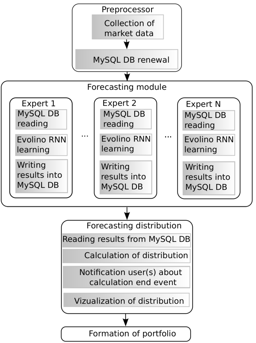
Fig. 2
Diagram of prediction module.
Figure
3 shows the basic operation of EVOLINO network Schmidhuber
et al. (
2007). The output of the network at time
$t,y(t)\in {\mathbb{R}^{2}}$ is computed by the following formulas
where
$u\in {\mathbb{R}^{2}}$ is
$k+1$ inputs,
$\phi (t)\in {\mathbb{R}^{2}}$ is the output of recurrent neural network
$\Phi (\cdot )$,
W is the weight matrix, which is calculated by mean square error minimization.
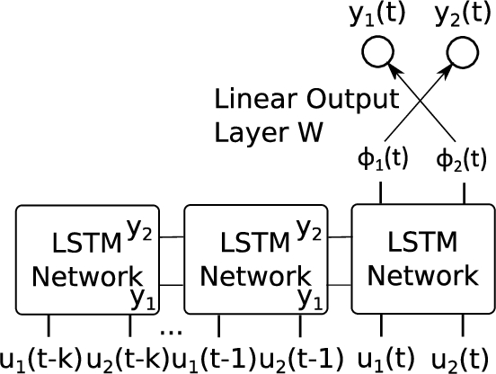
Fig. 3
Recurrent neural network receives sequential inputs $({u_{1}}(t-k),{u_{2}}(t-k))$ and creates outputs $({y_{1}}(t),{y_{2}}(t))$.
The block diagram of the LSTM network is shown in Fig.
4. The LSTM RNN forms network with
$N=4n$ memory cells, where
N is the total number of neurons and
n is the number of memory cells. The genetic evolution algorithm is applied to weights of each quartet of memory cells separately. The cell with a forget gate (
${G_{F}}$) and gate (
${G_{I}}$) controls access to the cell by the external inputs that are summed into the Σ unit, and the output gate (
${G_{0}}$). Nodes Π represent the multiplication function and the linear regression Moore–Penrose pseudo-inverse method used to compute pseudo-inverse weights for the output (Schmidhuber
et al. (
2005a),
2005b;
2007).
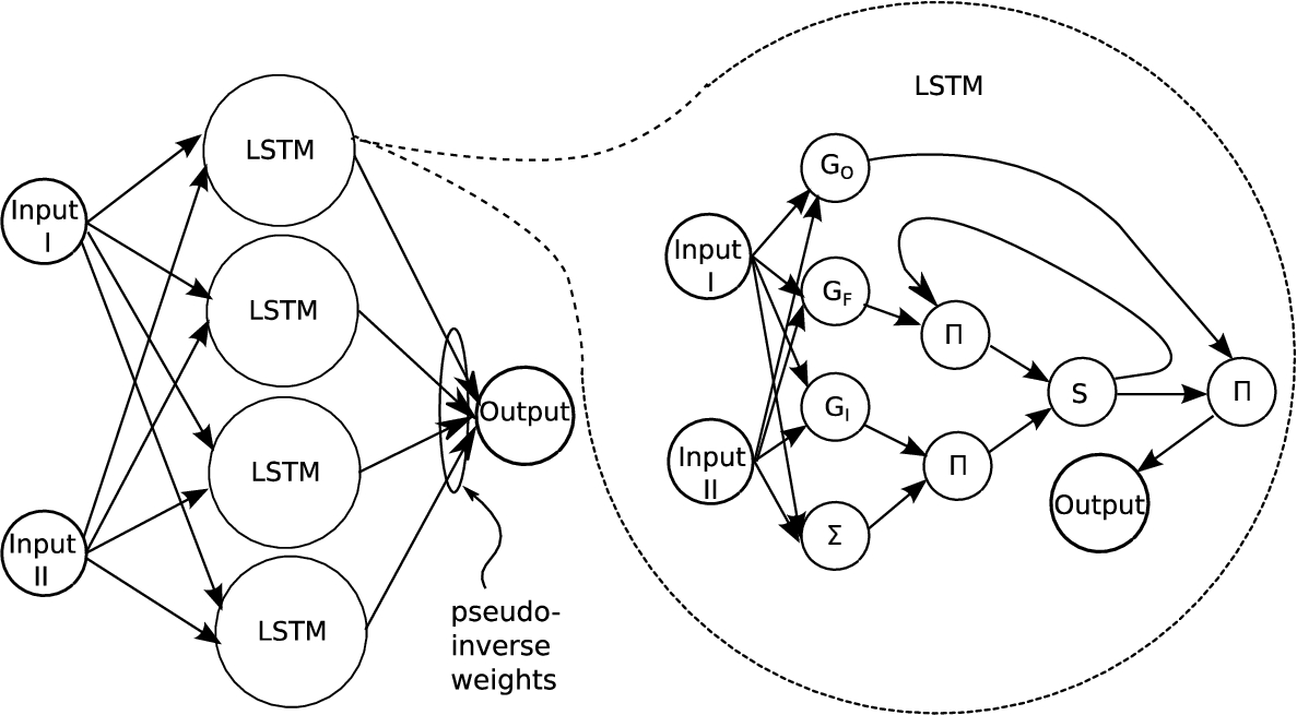
Fig. 4
LSTM network with four memory cells.
As described in Schmidhuber
et al. (
2007), the state of the cell
i is computed by
where
${g_{i}^{\mathit{in}}}$ and
${g_{i}^{\mathit{forget}}}$ are the activation of the input and forget gates, respectively, and
$\mathit{net}$ is the weighted sum of the external inputs (included by the
${\Sigma _{s}}$ in Fig.
4):
where
h is the identity function, and
${c_{j}}$ is the output of cell
j:
where
${g^{\mathit{out}}}$ is the output gate of cell
j. The value of each gate
${g_{i}}$ of memory cell
i is open or closed at time
t is calculated by:
where
type can be
input,
output, or
forget, and
σ is standard sigmoid function. The gates receive input from the output of other cell
${c_{j}}$ and from the external inputs to the network.
To date, the design of neural networks is more of an art than a science and is based on simulations derived from limited experiments Zang
et al. (
1998). Simulations of EVOLINO show that the best observable RMSE can be obtained for the configuration of neurons 36 and number of data 85 and equals 0.078 and second best RMSE 0.097 obtainable for configuration of neurons 64 and number of data 85. An investigation of training RMSE shows that it is in the interval from 0.0001 to 0.005 for number of neurons 60–64 and goes to
$1.3\times {10^{-29}}$ for number of neurons 68. Therefore, we use number of neurons 64. The number of training epochs is important also. It was chosen so that over-fitting of RNN would be avoided and would be equal to 180. All numeric data was obtained for tanh activation function.
The second idea of artificial prediction is based on uncertainty of the future events. This means that the future can be described by the distribution of different event, not trying to fix a single point in the future. This was taken into account by our algorithm using single predictions of RNNs to obtain the predicted histogram of possible exchange rate values. Additionally, we require to filter out unrealistic values. In this case, the first-fourth percentile method was used for removing values in this range as unrealistic.
Finally, weekly and daily histograms of possible exchange rate values were used for making decisions about appropriate investments. As was mentioned before, this method can be used because the weights are optimized using a genetic algorithm, where each optimization sequence gives different values for a single prediction point.
2.2 Data Preparation
The choice of exchange rates for trading is based on the orthogonality of the portfolio. The conditions under which an investment portfolio solves the efficient portfolio optimization problem are formulated by Roll (
1980). An orthogonal portfolio should satisfy the following conditions:
where
${r_{ij}}$ is the correlation coefficient between tools,
${\sigma _{i}}$ and
${\sigma _{j}}$ is the standard deviation of tool
i and
j, respectively.
It is very difficult to reach
${O_{c}}=0$ in practice. So, we use
ε to denote the degree of closeness to orthogonality:
Table 1
Exchangerates used in the investigation.
| Exchange rate names |
Abbreviation |
Time |
| British pounds and Australian dollars |
GBP/AUD |
D, W OHLC, NY, UK |
| New Zealand dollars and Canadian dollars |
NZD/CAD |
D, W OHLC, NY, UK |
| Euro and Japanese yen |
EUR/JPY |
D, W OHLC, NY, UK |
| US dollars and Swiss francs |
USD/CHF |
D, W OHLC, NY, UK |
| Euro and US dollars |
EUR/USD |
D, W OHLC, NY, UK |
| Gross Britain Pounds and US dollars |
GBP/USD |
D, W OHLC, NY, UK |
| US dollars and Swiss francs |
USD/CHF |
D, W OHLC, NY, UK |
| US dollars and Japanese yen |
USD/JPY |
D, W OHLC, NY, UK |
In our research, we use the following exchange rates: The daily (D) and weekly (W) open, high, low and close (OHLC) and the New York (NY) and London (UK) time exchange rates are recorded in a MySQL database Widenius
et al. (
2002). Additionally, we collect and use the XAU/USD rate (gold against the US dollar). The closest orthogonality of two data vectors ‘pupil and teacher’ can be achieved by varying time shift parameter
$a\geqslant 0$ while seeking a minimum of the sum Maknickas and Maknickienė (
2012):
The best shift value
a is then saved in the DB. Note that we do not use the direct
${\eta _{\mathit{XXX}/\mathit{YYY}}^{t}}$ exchange rate data (where index
$XXX/YYY$ denotes currency exchange rates GBP/AUD, NZD/CAD, EUR/JPY, USD/CHF, EUR/USD, GBP/USD, USD/CHF, USD/JPY), but the following rational logarithms of
${\eta _{i}^{t}}$ and
${\eta _{i}^{t-1}}$:
The choice of the logarithmic scale was based on a lognormal distributed data of the current investigation. So, a neural network will optimize weights for logarithmic, time percentage growth/decrease of exchange rate values. When the best four different shift values have been determined, the evolutionary LSTM RNN can begin the weight optimization process. RNN input data must be in the range
$[0,1]$, so the original data should be normalized by dividing all set of values by the maximum value in the interval
$[0,T]$, i.e.
The predicted data should be reversed by an opposite algorithm using the same value of
${l_{\max }^{j}}$. All predicted exchange rate values are multiplied by max value
${l_{\max }^{j}}$. Finally, the exponent of each predicted value is applied as follows:
where
${\eta _{j}^{0}}$ is the first value in the set.
2.3 Acceleration of Simulation
Selection of the optimal number in an ensemble was investigated in an earlier work Maknickienė and Maknickas (
2013). Two types of acceleration were applied in this work: software based and hardware based.
The pyhton profiler was used for software based acceleration. The profiler shows time consumption of running functions. The obtained running times of pure python functions allow to identify functions which must be accelerated. The slowest running functions then were converted into fortran code and after compilation by f2py Peterson (
2009) were imported into EVOLINO python code. Conversion of python code to fortran code allows an acceleration from 10 to 100 times.
Hardware acceleration is achieved using a multi-core workstation by applying the MPI python interface MPI4PY (Dalcin
et al. (
2011),
2008;
2005). The calculations were performed in parallel on the dedicated server of www.hostex.lt cloud with the following configuration: cpu is 32x Intel(R) Xeon(R) CPU E5-2630 v3 @ 2.40 GHz; ram is 64 GB RAM; hdd is RAID1 600 GB SAS. An ensemble of 176 predictive neural networks on the presented configurations allows one to obtain forecasting in a half hour (20–30 min). Finally, the support system generates the prediction histogram and its parameters such as the mean, median, mode, skewness and kurtosis.
2.4 Investment Asset Allocation
In general, selection of the investment portfolio and diversification of investment risk can be done by using Markowitz (
1952) portfolio optimization equations
where
${R_{i}}$ is the return on asset
i and
${\omega _{i}}$ is the weighting of component asset (that is, the proportion of asset
i in the portfolio),
${\sigma _{i}}$ is the return variance of asset component
i and
${\rho _{ij}}$ is the correlation coefficient between the returns on asset components
i and
j. If the return variance of asset components is known, the optimization can be done by quadratic programming algorithms.
It can be demonstrated that the minimum of total return variance is close to
${\textstyle\sum _{i}}{\omega _{i}^{2}}{\sigma _{i}^{2}}$ Maknickienė (
2014). Therefore, the minimum can be achieved by choosing large enough amount of asset components or by choosing of small amount of orthogonal asset components. Furthermore, obtained forecasting distributions allow to calculate the probability of sell or buy orders for a current market exchange rate by summation of forecasting distribution from the current exchange rate to zero or to max value, accordingly. It allows to determine which direction the asset component must be traded. If total buy or sell probability of the asset component return is near 1, we have a strong
buy or
sell signal. On the other hand, if total buy or sell probability of an asset component return is near 0.5, we have a strong
hold signal. Finally, we will use the equation
for the determination of weights
${\omega _{i}}$, where
${p_{\mathit{ri}}}$ is the probability of asset component return without solving quadratic programming optimization equations.
3 Trading Strategies
The information that is available to the investor in the currency market is highly diverse. The proper selection of information channels, data and strategies can significantly increase the probability of successful transactions. The predicted multi-modal distribution provides useful information for investors. The standard deviation indicates the riskiness of a decision, the kurtosis reflects the dispersal of possible values and the skewness additionally indicates the asymmetry of the decision. Furthermore, second and third modes also provide information about changes in the future exchange rate value.
Verification is made in real-time with the demo platform of ‘Oanda’ by using seven different portfolios with different exchange rates: NZD/CAD (New Zealand dollars and Canadian dollars), EUR/JPY (Euro and Japanese yen), GBP/AUD (British pounds and Australian dollars), USD/CHF (US dollars and Swiss francs), USD/JPY (US dollar and Japanese yen), EUR/USD (Euro and US dollars) and GBP/USD (British pounds and US dollars). Our research compares four different strategies based on the combination of distribution forecasting: high-low, day-week, UK-NY end high-low-UK-NY.
3.1 High-Low Strategy
The historical data consist of high, low, and open, closing values, so the distribution of expected values predicts the corresponding exchange rate for the next period. However, close or open data are less informative for investors. Obviously, an investor makes profit on his decision to buy the lowest values and sell the highest values of financial instruments. Thus, our proposal is to use for the prediction assessment the composition of two distributions, one of which produced using low exchange rate values and the other using high exchange rate values. Thus, our support system is predicting twice. The assessment is made from the composition of high-low distributions, taking into account the close values of the previous day. So, real time decisions are made according to the exchange rate value at the moment of decision-making Stankevic˘ienė
et al. (
2014).
An example of a high-low assessment is shown in Fig.
5, which presents the two distributions for the expected EUR/JPY values: high (black) and low (grey). The modes of these distributions are to the right of the close values (the dotted line), so the trading decision in these cases is to
buy. For this exchange rate
buy trading decision, the probability of buy loss
${P_{l}}=0.22$, and the probability of buy profit
${P_{p}}=0.78$, where the probability is calculated as normed sum of bars below and above close value.
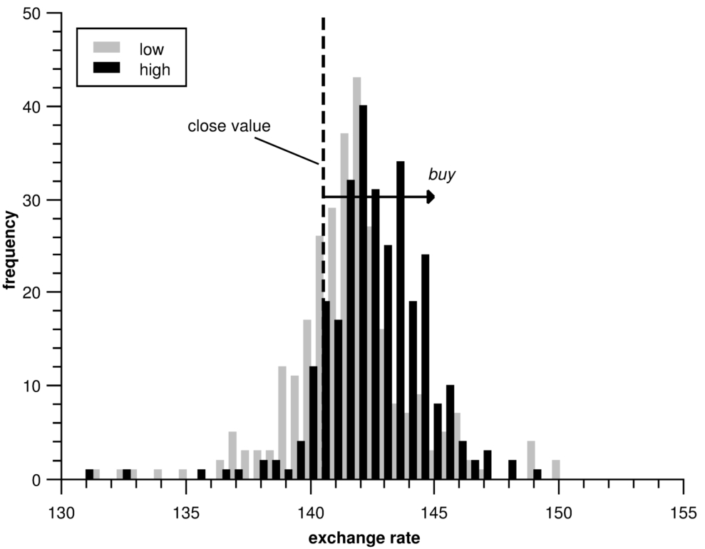
Fig. 5
High-low distributions of daily EUR/JPY predicted exchange rate.
The high-low strategy helps decision-makers in the exchange markets to recognize signals of transactions and to fix limits for expectations (take a profit and stop a loss).
3.2 Daily-Weekly-High-Low Strategy
A short-term prediction is useful for quickly making decisions in real-time speculations. Knowledge about long-term predictions is the basis for a trading strategy. A combination of these predictions gives a new time horizon for investors and makes their decisions more strategic.
The support system is used four times in this case: daily historical data with high values, daily data with low values, weekly data with high values and weekly data with low values. Two compositions of distributions have some variants. When both compositions are showing the markets changing in the same direction, it is a very clear market trend, but when the two compositions show the markets changing in different directions, the markets are in state of uncertainty.
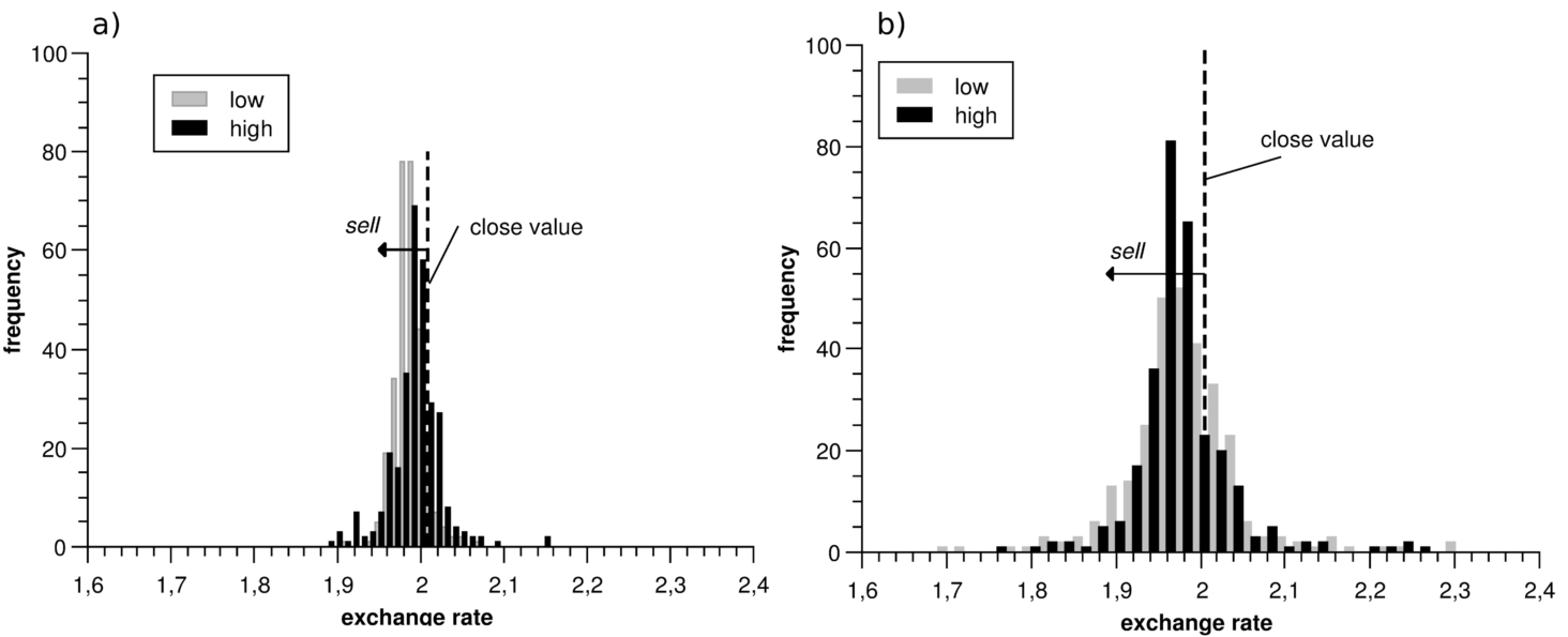
Fig. 6
Daily (a) and weekly (b) GBP/AUD high-low compositions of distributions in one scale.
Our experiment seeks to compare two high-low compositions based on daily and weekly time series, where short-term predictions were made using historical data on daily highs and lows. There we can see the decision to
sell because both distributions (black and grey) are on the left side of the closing value (the dotted line) of the previous day. The probability of sell profit
${P_{p}}$ is
${P_{p}}=0.89$, probability of sell loss
${P_{l}}$ is
${P_{l}}=0.11$, where probability is calculated as a normed sum of bars below and above close value. Therefore in the case of the daily GBP/AUD predicted exchange rate distributions the
sell trading decision should be made. Weekly exchange rates predictions are made in the same way. The weekly composition of probabilities is similar, and the decision is also to
sell. The probability of loss
${P_{l}}$ is
${P_{l}}=0.22$ and the probability of profit
${P_{p}}$ is
${P_{p}}=0.78$, where the same way probability is calculated as a normed sum of bars below and above close value. Therefore in the case of the weekly predicted distributions of GBP/AUD the
sell trading decision should be made, too. A comparison of daily and weekly GBP/AUD predictions is shown in Fig.
6. The comparison of daily and weekly compositions of distributions in one scale shows that the weekly distribution is more scattered, so it is more risky. But information from daily and weekly predictions helps investors to make daily transactions by knowing the perspective of a week. Sometimes the directions of daily and weekly predictions are the same, and sometimes they are the opposite.
3.3 UK-NY Strategy
The global finance market has, in general, no time zones. All exchange rates are the same around the globe. Divisions of historical data into time intervals are different in the London exchange market (UK) and in the New York exchange market (NY). The shift of time is equal to five hours. We decided to build a composition of forecasts from two distributions of UK-NY. An expectation of this strategy is to go profitable by using daily exchange rates.
In this case, the support system is used twice: the first time with data fixed at the moment of the closing of the London exchange market and the second time with data fixed at the moment of the closing of the New York exchange market. The results of the prediction are composed of two distributions, which show the direction of the exchange rate changing during the period of the New York trading hours. Therefore, the decision should be made at the moment of opening hours of the New York trading time.
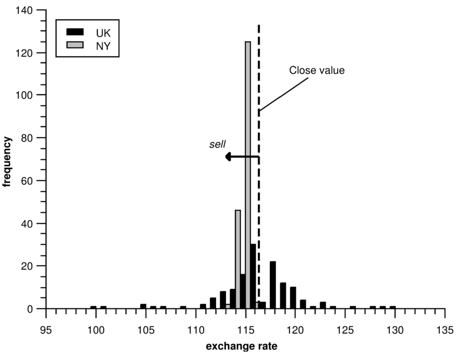
Fig. 7
Distributions of UK-NY of daily USD/JPY exchange rate predictions.
The distributions combined by UK-NY time difference for USD/JPY rate expected values are shown in Fig.
7. There is a clear shift of expectations to the right side, so the decision is to
sell. A short-term prediction can be successfully used for daily trading. A trading decision is made with the newest information of the finance market. The shift of time in five hours allows investors to recognize the signals of the market in a very short time.
3.4 High-Low-UK-NY Strategy
For investors in exchange markets, it is important to know not only the direction of exchange of the exchange rate but also the moment when this trend will change. To find the limits of daily fluctuations of the exchange rate, we decided to use high-low-UK-NY distributions. A combination of high-low and UK-NY predictions can be explained like 3D: high-low-shift.
The support system in this case is used four times: separately high and low historical data fixed at the moment of the closing of the London market and separately high and low historical data fixed at the moment of the closing of the New York market. Two compositions of distributions determine the shift of exchange rate and the limits of the trading day in the future: high and low.
Cases of EUR/USD high-UK-NY and low-UK-NY are shown in Fig.
8. There we can see the decision is to buy because the modes of both compositions of distributions (high and low) are on the right side from the closing value (the dotted line) of the previous day, and the distributions of NY are to the right of UK distributions. The modes of the distributions are as follows: low-UK 1.11, low-NY 1.12, high-UK 1.115, high-NY 1.122. The close value of the previous day is 1.11068, and Take profit can be fixed at 1.12.
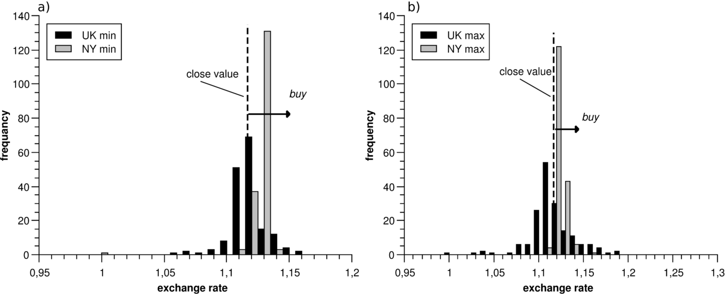
Fig. 8
Low-UK-NY composition of distributions: (a) and high-UK-NY composition of distributions, (b) of daily EUR/USD exchange rate predictions.
The comparison of high-UK-NY and low-UK-NY compositions of distributions in one scale shows that the UK distributions are more scattered, so the UK market is more risky. However, information from the forecasts from two time zones helps investors make daily decisions while knowing the perspective of the full day. Sometimes the directions of high and low forecasts are the same, and sometimes they are opposite, which is additional information about the behaviour of the exchange markets.
3.5 Evaluation of Prediction Strategies
The distribution of expected values is also a distribution of point predictions. An investor using probability distribution, selects one point from the distribution for take profit and another for stop loss. So we decided to evaluate our new strategies by using the mean absolute percentage error (MAPE).
Table 2
Trading results using different portfolios.
| Strategy |
Portfolio |
MAPE |
Total profit |
Profit |
|
(level of risk) |
(%) |
(euro) |
per trade |
| Hi |
daily moderate |
0.20 |
3612.29 |
26.23 |
| gh-low |
conservative |
0.3 |
1041.82 |
12.39 |
|
daily aggressive |
0.38 |
2855.29 |
11.25 |
| Day-week |
conservative |
0.37 |
1777.15 |
44.4 |
|
moderate |
0.32 |
2219.0 |
34.7 |
|
aggressive |
0.86 |
2934.04 |
22 |
| NY-UK |
conservative |
0.10 |
741.53 |
41.2 |
The best evaluator of forecasting the finance markets is the real market with all of its unpredictable factors like banking interventions, geopolitical events, natural catastrophes and other events. We are trading every day on the ‘Oanda’ demo platform with seven different portfolios with different level of risk. Portfolios are determined by the choice of different risk levels of the trading account. A conservative portfolio has a 1:10 leverage, and funds are shared equally. A moderate portfolio has a 1:20 leverage, and the funds are divided in proportion to the projected profit. An aggressive portfolio has a 1:50 leverage, and the funds are divided in proportion to the projected profit. Different strategies started at different times: high-low has been alive more than one year, day-week has been alive slightly less than one year, UK-NY has been alive for some months, and high-low-UK-NY is too new for evaluation.
The MAPE varies from 0.1% to 0.86%. The profitability is similar with regard to the duration of trading in the currency market. Moderate and aggressive portfolios are more profitable than conservative ones. Profit per trade is about twice as high when applied daily-weekly or with the UK-NY strategy than in the case of the high-low strategy. These results show that the daily-weekly and UK-NY strategies allow investors to find a more accurate time for stopping transactions and keep the currency active for a longer period of time.
4 Conclusions
In our research, we developed a novel support system by using the latest technological breakthroughs of artificial intelligence and investor experience. A combination of distributional forecasts gives investors new opportunities based on data mining and information about future behaviour of exchange rates.
We validated the efficiency of developed trading support system by calculation of predicting RMSE of single agent of EVOLINO RNN ensemble in comparison to predicting RMSE of Mackey–Glass chaotic time series. The numeric recalculation of different RNN configurations allows to find the optimized configuration neural networks of predicting module.
We proposed four different strategies based on a combination of distribution forecasts with different opportunities of time perspective and fixing the end of transactions:
-
1. The high-low strategy helps investors to recognize signals of transactions and to fix limits for expectations;
-
2. The daily-weekly strategy helps investors to make daily transactions while knowing the perspective of a week;
-
3. The UK-NY strategy allows investors to recognize the signals of the market in a very short term;
-
4. The high-low-UK-NY strategy helps investors to recognize the signals of transactions in a very short term and to fix the limits.
The accuracy of forecasting MAPE with respect to mode in all cases is from 0.1% to 0.86%. The profitability is similar with regard to the duration of trading in the currency market. Profit per trade is about twice as high when applied daily-weekly or with the UK-NY strategy than in the case of the high-low strategy. These results show that daily-weekly and UK-NY strategies allow the investor to find a more accurate time for stopping a transaction and keeping the currency active for a longer period of time.

