Informatica logo


Login Register

  1. Home
  2. Issues
  3. Volume 35, Issue 2 (2024)
  4. Proportional Fuzzy Set Extensions and Im ...

Proportional Fuzzy Set Extensions and Imprecise Proportions
Volume 35, Issue 2 (2024), pp. 311–339
Cengiz Kahraman  

Authors

 
Placeholder
https://doi.org/10.15388/24-INFOR550
Pub. online: 29 March 2024      Type: Research Article      Open accessOpen Access

Received
1 November 2023
Accepted
1 March 2024
Published
29 March 2024

Abstract

The extensions of ordinary fuzzy sets are problematic because they require decimal numbers for membership, non-membership and indecision degrees of an element from the experts, which cannot be easily determined. This will be more difficult when three or more digits’ membership degrees have to be assigned. Instead, proportional relations between the degrees of parameters of a fuzzy set extension will make it easier to determine the membership, non-membership, and indecision degrees. The objective of this paper is to present a simple but effective technique for determining these degrees with several decimal digits and to enable the expert to assign more stable values when asked at different time points. Some proportion-based models for the fuzzy sets extensions, intuitionistic fuzzy sets, Pythagorean fuzzy sets, picture fuzzy sets, and spherical fuzzy sets are proposed, including their arithmetic operations and aggregation operators. Proportional fuzzy sets require only the proportional relations between the parameters of the extensions of fuzzy sets. Their contribution is that these models will ease the use of fuzzy set extensions with the data better representing expert judgments. The imprecise definition of proportions is also incorporated into the given models. The application and comparative analyses result in that proportional fuzzy sets are easily applied to any problem and produce valid outcomes. Furthermore, proportional fuzzy sets clearly showed the role of the degree of indecision in the ranking of alternatives in binomial and trinomial fuzzy sets. In the considered car selection problem, it has been observed that there are minor changes in the ordering of intuitionistic and spherical fuzzy sets.

1 Introduction

Several new extensions of ordinary fuzzy sets appear in the literature every year. Starting with type-2 fuzzy sets (Zadeh, 1975), all the other fuzzy set extensions, such as intuitionistic fuzzy sets (IFS) (Atanassov, 1986, 1989, 1999), fuzzy multisets (Yager, 1986), neutrosophic sets (Smarandache, 1998), nonstationary fuzzy sets (Garibaldi and Ozen, 2007), hesitant fuzzy sets (Torra, 2010), Pythagorean fuzzy sets (PyFS) (Yager, 2013), picture fuzzy sets (PiFs) (Cuong and Kreinovich, 2013), q-rung orthopair fuzzy sets (Yager, 2016), spherical fuzzy sets (SFS) (Kahraman and Kutlu Gündogdu, 2018; Kutlu Gündoğdu and Kahraman, 2019), fermatean fuzzy sets (Senapati and Yager, 2020), circular intuitionistic fuzzy sets (Atanassov, 2020), cognitive fuzzy sets (Jiang and Liao, 2020) decomposed fuzzy sets (Cebi et al., 2022), and continuous intuitionistic fuzzy sets (Alkan and Kahraman, 2023) try to model human thoughts by using more parameters in different ways. All these extensions require decimal membership degrees with two or more decimal places to be assigned by experts, which is generally a tedious process for them. The use of a larger number of parameters with fuzzy set extensions makes it more difficult to determine their values with decimal numbers and reduces the possibility of assigning correct membership values. It is a high possibility for experts to assign different decimal membership degrees to the same element of a fuzzy set at different points of time in short intervals. Consider the proposition “the numbers around X are larger than the numbers around Y”. When you ask experts to assign a degree for the truthfulness (membership), they will generally assign decimal numbers with one decimal place, such as 0.6 or 0.8, since it is difficult to correctly determine these degrees with two or more decimal places without using a technique. This challenge is solved using a technique based on proportional relations between the degrees. This paper proposes an easy but effective way to determine the values of membership, non-membership, and indecision degrees. The contribution of the paper is the application of this technique to the most used fuzzy set extensions and the demonstration of how to apply them in decision making problems.
The similar problem has been handled by some researchers in different ways (Atanassov et al., 2010; Dalkılıç, 2021). Determination of a membership function hugely depends on problem size and context of the problem. Relying on personal intuition and experience of the researchers/individuals, it becomes quite challenging to exclude the inherent uncertainties in this process (Chowdhury and Kar, 2020). Hasan and Sobhan (2020) describe a new and simple way of constructing fuzzy membership function by using five different data sets. If there is any outlier in the data set, it is detected by the proposed method by using a box plot. This study provides a suggestion that will greatly reduce this difficulty. Instead of trying to determine decimal values, the expert can inform his/her opinions about the proportions between the parameters. This will enable assigning easier and more accurate degrees. Consider the eagle in Fig. 1. How long is its wing? What is its tail length? What is the length from the top of the eagle’s head to its feet?
infor550_g001.jpg
Fig. 1
An eagle.
Without using a meter, answering these questions is really hard. But we can state that the wing length of the eagle is about three times its tail’s length and the wing length of the eagle is about 1.5 times the length from the top of the eagle’s head to its feet. If we can state such proportions, then the problem can be solved by more correct and objective data than with the estimated metric measurements.
In this paper, proportional fuzzy sets (PFS) are developed to represent a vague and imprecise definition of membership parameters and to develop proportional fuzzy set extensions such as proportional intuitionistic fuzzy sets and proportional picture fuzzy sets. This new way to determine membership, non-membership and indecision degrees is easier and more correct than the direct assignment of a decimal membership degree. PFS hypothesis is that humans can better express their judgments by using proportional judgments instead of decimal membership degree judgments. For instance, let an expert assign a picture fuzzy number $\langle x;\mu ,\pi ,\vartheta \rangle $ for the proposition “it is very cold today”. Assume that the expert assigns $\langle 0.625,0.125,0.250\rangle $ which corresponds a membership degree of 0.625, an indecision degree of 0.125, and a non-membership degree of 0.250. It is a difficult process to assign these degrees correctly using decimal values whereas it is easier to make a judgment, such as a membership degree relatively 5 times larger than hesitancy and a non-membership degree relatively 2 times larger than hesitancy. Proportional fuzzy sets extensions are based on the fact that relative proportions give us the required degrees easily, simply and correctly. Thus, a PFS number can be represented by $\langle x;{k_{\pi \mu }},{k_{\pi \vartheta }}\rangle $. The arithmetic operations and aggregation operators of PFS are presented for proportional IFS, proportional PyFS, proportional PiFS, and proportional SFS.
In this paper, imprecise proportions such as “around 2.5” or “between 3.5 and 4” are also handled to show how to model them in arithmetic operations and aggregation operators. Triangular and trapezoidal membership functions of proportions are considered for the mentioned four fuzzy sets extensions.
The rest of the paper is organized as follows. Section 2 introduces the preliminaries of proportional fuzzy sets and develops the proportional fuzzy set extensions. Section 3 includes the incorporation of imprecise proportions to the developed PFS extensions. Section 4 gives the applications of the developed PFS extensions on MCDM problems. Section 5 concludes the paper with discussions and future research directions.

2 Proportional Fuzzy Sets (PIFS)

In this section, we introduce proportional fuzzy set extensions. We first present the basic equations for each PFS extension, then give their arithmetic operations and aggregation operators.

2.1 Proportional Intuitionistic Fuzzy Sets

Consider the intuitionistic fuzzy set $\tilde{A}=\{\langle x;{\mu _{\tilde{A}}}(x),{\vartheta _{\tilde{A}}}(x)\rangle \hspace{0.1667em}|\hspace{0.1667em}x\epsilon X\}$. Assume that the expert judges the proportions between $\mu (x)$ and $\vartheta (x)$ based on the hesitancy degree $\pi (x)$ in his/her mind as in Eqs. (1) and (2):
(1)
\[ \mu (x)={k_{1}}{\pi _{\tilde{A}}}(x)\]
and
(2)
\[ \vartheta (x)={k_{2}}{\pi _{\tilde{A}}}(x)\]
satisfying
(3)
\[ {\pi _{\tilde{A}}}(x)+{k_{1}}{\pi _{\tilde{A}}}(x)+{k_{2}}{\pi _{\tilde{A}}}(x)=1\]
and
(4)
\[ {\pi _{\tilde{A}}}(x)=\frac{1}{1+{k_{1}}+{k_{2}}}.\]
Then, each element in the set $\tilde{A}$ can be represented by
(5)
\[ \tilde{A}=\bigg\{\bigg\langle x;{k_{1}}\frac{1}{1+{k_{1}}+{k_{2}}},{k_{2}}\frac{1}{1+{k_{1}}+{k_{2}}}\bigg\rangle \hspace{0.1667em}\Big|\hspace{0.1667em}x\in X\bigg\}\]
with a hesitancy degree of $\frac{1}{1+{k_{1}}+{k_{2}}}$.
For instance, consider the proposition “${P_{0}}$: Electric vehicles are problematic in cold weather”. The expert believes that the membership (truthfulness) degree of the proposition is two times larger than indecision (hesitancy) degree and the non-membership (falsity) degree is five times larger than the indecision degree in expert’s mind. Then, based on Eq. (5), the intuitionistic fuzzy set can be written as $\langle {P_{0}};0.250,0.625\rangle $.
It should be also indicated that $(2,5)$ is not equal to a proportion of $(4,10)$ since their corresponding membership degrees are quite different.
Thus, a proportional intuitionistic fuzzy set ${\tilde{A}_{P}}$ can be represented by Eq. (6):
(6)
\[ {\tilde{A}_{P}}=\big\{\langle x;{k_{\pi 1}},{k_{\pi 2}}\rangle \hspace{0.1667em}\big|\hspace{0.1667em}x\in X\big\}.\]
Addition and multiplication operations are defined as in Eqs. (7)–(8), respectively.
(7)
\[\begin{aligned}{}\tilde{A}+\tilde{B}& =\bigg(x;{k_{A1}}\frac{1}{1+{k_{A1}}+{k_{A2}}}+{k_{B1}}\frac{1}{1+{k_{B1}}+{k_{B2}}}-{k_{A1}}\frac{1}{1+{k_{A1}}+{k_{A2}}}\\ {} & \hspace{1em}\times {k_{B1}}\frac{1}{1+{k_{B1}}+{k_{B2}}},\frac{1}{1+{k_{A1}}+{k_{A2}}}\\ {} & \hspace{1em}\times \frac{1}{1+{k_{B1}}+{k_{B2}}},{k_{B2}}\frac{1}{1+{k_{B1}}+{k_{B2}}}\times {k_{A2}}\frac{1}{1+{k_{A1}}+{k_{A2}}}\hspace{0.1667em}\Big\rfloor \hspace{0.1667em}x\in X\bigg),\end{aligned}\]
(8)
\[\begin{aligned}{}\tilde{A}\times \tilde{B}& =\bigg(x;{k_{A1}}\frac{1}{1+{k_{A1}}+{k_{A2}}}\times {k_{B1}}\frac{1}{1+{k_{B1}}+{k_{B2}}},\frac{1}{1+{k_{A1}}+{k_{A2}}}\\ {} & \hspace{1em}+\displaystyle \frac{1}{1+{k_{B1}}+{k_{B2}}}-\frac{1}{1+{k_{A1}}+{k_{A2}}}\times \frac{1}{1+{k_{B1}}+{k_{B2}}},{k_{B2}}\frac{1}{1+{k_{B1}}+{k_{B2}}}\\ {} & \hspace{1em}+\displaystyle {k_{A2}}\frac{1}{1+{k_{A1}}+{k_{A2}}}-{k_{B2}}\frac{1}{1+{k_{B1}}+{k_{B2}}}\times {k_{A2}}\frac{1}{1+{k_{A1}}+{k_{A2}}}\hspace{0.1667em}\Big|\hspace{0.1667em}x\in X\bigg).\end{aligned}\]
The multiplication by a constant and power operation are given by Eqs. (9)–(10), respectively.
(9)
\[\begin{aligned}{}& \lambda \cdot \tilde{A}=\bigg\langle 1-{\bigg(1-{k_{A1}}\frac{1}{1+{k_{A1}}+{k_{A2}}}\bigg)^{\lambda }},{\bigg({k_{A2}}\frac{1}{1+{k_{A1}}+{k_{A2}}}\bigg)^{\lambda }}\bigg\rangle ,\end{aligned}\]
(10)
\[\begin{aligned}{}& {\tilde{A}^{\lambda }}=\bigg\langle {\bigg({k_{A1}}\frac{1}{1+{k_{A1}}+{k_{A2}}}\bigg)^{\lambda }},1-{\bigg(1-{k_{A2}}\frac{1}{1+{k_{A1}}+{k_{A2}}}\bigg)^{\lambda }}\bigg\rangle .\end{aligned}\]
Definition 1.
Let ${\alpha _{j}}$ $(j=1,2,\dots ,n)$ be a collection of PIFNs. The proportional intuitionistic fuzzy weighted averaging (PIFWA) operator is a mapping ${\textit{PI}^{n}}\to \textit{PI}$ such that
(11)
\[ {\textit{PIFWA}_{w}}({\alpha _{1}},{\alpha _{2}},\dots ,{\alpha _{n}})={\underset{j=1}{\overset{n}{\bigoplus }}}({w_{j}}{\alpha _{j}}),\]
where $w={({w_{1}},{w_{2}},\dots ,{w_{n}})^{T}}$ is the weight vector of ${\alpha _{j}}$ $(j=1,2,\dots ,n)$ and ${w_{j}}\gt 0$, ${\textstyle\sum _{j=1}^{n}}{w_{j}}=1$. Then
(12)
\[\begin{aligned}{}& {\textit{PIFWA}_{w}}({\alpha _{1}},{\alpha _{2}},\dots ,{\alpha _{n}})\\ {} & \hspace{1em}=\Bigg(1-{\prod \limits_{j=1}^{n}}{\bigg(1-{k_{1j}}\frac{1}{1+{k_{1j}}+{k_{2j}}}\bigg)^{{w_{j}}}},{\prod \limits_{j=1}^{n}}{\bigg({k_{2j}}\frac{1}{1+{k_{1j}}+{k_{2j}}}\bigg)^{{w_{j}}}}\Bigg).\end{aligned}\]
Definition 2.
Let ${\alpha _{j}}$ $(j=1,2,\dots ,n)$ be a collection of PIFNs. The proportional intuitionistic fuzzy weighted geometric (PIFWG) operator is a mapping ${\textit{PI}^{n}}\to \textit{PI}$ such that
(13)
\[ {\textit{PIFWG}_{w}}({\alpha _{1}},{\alpha _{2}},\dots ,{\alpha _{n}})={\underset{j=1}{\overset{n}{\bigotimes }}}{({\alpha _{j}})^{{w_{j}}}},\]
where $w={({w_{1}},{w_{2}},\dots ,{w_{n}})^{T}}$ is the weight vector of ${\alpha _{j}}$ $(j=1,2,\dots ,n)$ and ${w_{j}}\gt 0$, ${\textstyle\sum _{j=1}^{n}}{w_{j}}=1$. Then
(14)
\[\begin{aligned}{}& {\textit{PIFWG}_{w}}({\alpha _{1}},{\alpha _{2}},\dots ,{\alpha _{n}})\\ {} & \hspace{1em}=\Bigg({\prod \limits_{j=1}^{n}}{\bigg({k_{1j}}\frac{1}{1+{k_{1j}}+{k_{2j}}}\bigg)^{{w_{j}}}},1-{\prod \limits_{j=1}^{n}}{\bigg(1-{k_{2j}}\frac{1}{1+{k_{1j}}+{k_{2j}}}\bigg)^{{w_{j}}}}\Bigg).\end{aligned}\]

2.2 Proportional Pythagorean Fuzzy Sets

Consider the Pythagorean fuzzy set $\tilde{P}=\{\langle x;{\mu _{\tilde{P}}}(x),{\vartheta _{\tilde{P}}}(x)\rangle \hspace{0.1667em}|\hspace{0.1667em}x\epsilon X\}$. Assume that the expert judges the proportions between ${\mu _{\tilde{P}}}(x)$ and ${\vartheta _{\tilde{P}}}(x)$ based on the hesitancy degree ${\pi _{P}}(x)$ in his/her mind as in Eqs. (15) and (16):
(15)
\[ {\mu _{\tilde{P}}}(x)={k_{1}}{\pi _{\tilde{P}}}(x)\]
and
(16)
\[ {\vartheta _{\tilde{P}}}(x)={k_{2}}{\pi _{\tilde{P}}}(x)\]
satisfying
(17)
\[ {\big({\pi _{P}}(x)\big)^{2}}+{\big({k_{1}}{\pi _{P}}(x)\big)^{2}}+{\big({k_{2}}{\pi _{P}}(x)\big)^{2}}=1\]
and
(18)
\[ {\pi _{P}}(x)=\sqrt{\frac{1}{1+{k_{1}^{2}}+{k_{2}^{2}}}}.\]
Then, each element in the set $\tilde{A}$ can be represented by
(19)
\[ \tilde{A}=\bigg\{\bigg\langle x;{k_{1}}\sqrt{\frac{1}{1+{k_{1}^{2}}+{k_{2}^{2}}}},{k_{2}}\sqrt{\frac{1}{1+{k_{1}^{2}}+{k_{2}^{2}}}}\bigg\rangle \hspace{0.1667em}\Big|\hspace{0.1667em}x\in X\bigg\}\]
with a hesitancy degree of $\sqrt{\frac{1}{1+{k_{1}^{2}}+{k_{2}^{2}}}}$.
For instance, consider the proposition “${P_{0}}$: Electric vehicles are problematic in cold weathers”. The expert believes that the membership (truthfulness) degree of the proposition is two times larger than indecision (hesitancy) degree and the non-membership (falsity) degree is five times larger than the indecision degree in expert’s mind. Then, based on Eq. (19), the Pythagorean fuzzy set can be written as $\langle {P_{0}};0.365148,0.912871\rangle $ with a hesitancy degree of 0.182574.
Thus the proportional intuitionistic fuzzy sets can be represented by Eq. (20):
(20)
\[ {\tilde{P}_{P}}=\big\{\langle x;{k_{\pi 1}};{k_{\pi 2}}\rangle \hspace{0.1667em}\big|\hspace{0.1667em}x\in X\big\}.\]
Let $\tilde{A}$ and $\tilde{B}$ be two Pythagorean fuzzy sets. Addition and multiplication operations are defined as in Eqs. (21)–(22), respectively.
(21)
\[\begin{aligned}{}& \tilde{A}+\tilde{B}\\ {} & \hspace{1em}=\Bigg(x;{k_{A1}}\sqrt{\frac{1}{1+{k_{A1}^{2}}+{k_{A2}^{2}}}}+{k_{B1}}\sqrt{\frac{1}{1+{k_{B1}^{2}}+{k_{B2}^{2}}}}-{k_{A1}}\sqrt{\frac{1}{1+{k_{A1}^{2}}+{k_{A2}^{2}}}}\\ {} & \hspace{2em}\times \displaystyle {k_{B1}}\sqrt{\frac{1}{1+{k_{B1}^{2}}+{k_{B2}^{2}}}},{k_{B2}}\sqrt{\frac{1}{1+{k_{B1}^{2}}+{k_{B2}^{2}}}}\times {k_{A2}}\sqrt{\frac{1}{1+{k_{A1}^{2}}+{k_{A2}^{2}}}}\hspace{0.1667em}\Big\rfloor \hspace{0.1667em}x\in X\Bigg),\end{aligned}\]
(22)
\[\begin{aligned}{}& \tilde{A}\times \tilde{B}\\ {} & \hspace{1em}=\Bigg(x,{k_{A1}}\sqrt{\frac{1}{1+{k_{A1}^{2}}+{k_{A2}^{2}}}}\times {k_{B1}}\sqrt{\frac{1}{1+{k_{B1}^{2}}+{k_{B2}^{2}}}},{k_{B2}}\sqrt{\frac{1}{1+{k_{B1}^{2}}+{k_{B2}^{2}}}}\\ {} & \hspace{2em}+\displaystyle {k_{A2}}\sqrt{\frac{1}{1+{k_{A1}^{2}}+{k_{A2}^{2}}}}-{k_{B2}}\sqrt{\frac{1}{1+{k_{B1}^{2}}+{k_{B2}^{2}}}}\times {k_{A2}}\sqrt{\frac{1}{1+{k_{A1}^{2}}+{k_{A2}^{2}}}}\hspace{0.1667em}\Big|\hspace{0.1667em}x\in X\hspace{-0.1667em}\Bigg)\end{aligned}\]
Assuming no refusal degree, the multiplication by a constant and power operation are given by Eqs. (23)–(24), respectively.
(23)
\[\begin{aligned}{}& \lambda \cdot \tilde{A}=\bigg\langle 1-{\bigg(1-{k_{A1}}\sqrt{\frac{1}{1+{k_{A1}^{2}}+{k_{A2}^{2}}}}\bigg)^{\lambda }},{\bigg({k_{A2}}\sqrt{\frac{1}{1+{k_{A1}^{2}}+{k_{A2}^{2}}}}\bigg)^{\lambda }}\bigg\rangle ,\end{aligned}\]
(24)
\[\begin{aligned}{}& {\tilde{A}^{\lambda }}=\bigg\langle {\bigg({k_{A1}}\sqrt{\frac{1}{1+{k_{A1}^{2}}+{k_{A2}^{2}}}}\bigg)^{\lambda }},1-{\bigg(1-{k_{A2}}\sqrt{\frac{1}{1+{k_{A1}^{2}}+{k_{A2}^{2}}}}\bigg)^{\lambda }}\bigg\rangle .\end{aligned}\]
Definition 3.
Let ${\alpha _{j}}$ $(j=1,2,\dots ,n)$ be a collection of PPFNs. The proportional picture fuzzy weighted averaging (PPFWA) operator is a mapping ${\textit{PP}^{n}}\to \textit{PP}$ such that
(25)
\[ {\textit{PPFWA}_{w}}({\alpha _{1}},{\alpha _{2}},\dots ,{\alpha _{n}})={\underset{j=1}{\overset{n}{\bigoplus }}}({w_{j}}{\alpha _{j}}),\]
where $w={({w_{1}},{w_{2}},\dots ,{w_{n}})^{T}}$ is the weight vector of ${\alpha _{j}}$ $(j=1,2,\dots ,n)$ and ${w_{j}}\gt 0$, ${\textstyle\sum _{j=1}^{n}}{w_{j}}=1$. Then
(26)
\[\begin{aligned}{}& {\textit{PPFWA}_{w}}({\alpha _{1}},{\alpha _{2}},\dots ,{\alpha _{n}})\\ {} & \hspace{1em}=\Bigg(1-{\prod \limits_{j=1}^{n}}{\bigg(1-{k_{1j}}\sqrt{\frac{1}{1+{k_{1j}^{2}}+{k_{2j}^{2}}}}\bigg)^{{w_{j}}}},{\prod \limits_{j=1}^{n}}{\bigg({k_{2j}}\sqrt{\frac{1}{1+{k_{1j}^{2}}+{k_{2j}^{2}}}}\bigg)^{{w_{j}}}}\Bigg).\end{aligned}\]
Definition 4.
Let ${\alpha _{j}}$ $(j=1,2,\dots ,n)$ be a collection of PPiFNs. The proportional picture fuzzy weighted geometric (PPiFWG) operator is a mapping ${\textit{PP}^{n}}\to \textit{PP}$ such that
(27)
\[ {\textit{PPFWG}_{w}}({\alpha _{1}},{\alpha _{2}},\dots ,{\alpha _{n}})={\underset{j=1}{\overset{n}{\bigotimes }}}{({\alpha _{j}})^{{w_{j}}}},\]
where $w={({w_{1}},{w_{2}},\dots ,{w_{n}})^{T}}$ is the weight vector of ${\alpha _{j}}$ $(j=1,2,\dots ,n)$ and ${w_{j}}\gt 0$, ${\textstyle\sum _{j=1}^{n}}{w_{j}}=1$. Then
(28)
\[\begin{aligned}{}& {\textit{PPFWG}_{w}}({\alpha _{1}},{\alpha _{2}},\dots ,{\alpha _{n}})\\ {} & \hspace{1em}=\Bigg({\prod \limits_{j=1}^{n}}{\bigg({k_{1j}}\sqrt{\frac{1}{1+{k_{1j}^{2}}+{k_{2j}^{2}}}}\bigg)^{{w_{j}}}},1-{\prod \limits_{j=1}^{n}}{\bigg(1-{k_{2j}}\sqrt{\frac{1}{1+{k_{1j}^{2}}+{k_{2j}^{2}}}}\bigg)^{{w_{j}}}}\Bigg).\end{aligned}\]

2.3 Proportional Picture Fuzzy Sets

Consider the picture fuzzy set $\tilde{T}=\{\langle x;{\mu _{\tilde{T}}}(x),{\pi _{\tilde{T}}}(x),{\vartheta _{\tilde{T}}}(x)\rangle \hspace{0.1667em}\big|\hspace{0.1667em}x\epsilon X\}$. Assume that the expert judges the proportions between ${\mu _{\tilde{T}}}(x)$, ${\vartheta _{\tilde{T}}}(x)$ and ${\pi _{\tilde{T}}}(x)$ as in Eqs. (29)–(30) (Kahraman, 2024):
(29)
\[ \mu (x)={k_{1}}{\pi _{\tilde{T}}}(x)\]
and
(30)
\[ \vartheta (x)={k_{2}}{\pi _{\tilde{T}}}(x)\]
satisfying
(31)
\[ {\pi _{\tilde{T}}}(x)+{k_{1}}{\pi _{\tilde{T}}}(x)+{k_{2}}{\pi _{\tilde{T}}}(x)+{r_{\tilde{T}}}(x)=1.\]
The refusal degree can be given by Eq. (32)
(32)
\[ {r_{\tilde{T}}}(x)=1-\big({\pi _{\tilde{T}}}(x)+{k_{1}}{\pi _{\tilde{T}}}(x)+{k_{2}}{\pi _{\tilde{T}}}(x)\big)\]
and
(33)
\[ {\pi _{\tilde{T}}}(x)=\frac{1-{r_{\tilde{T}}}(x)}{1+{k_{1}}+{k_{2}}}.\]
Then, each element in the set $\tilde{T}$ can be represented by
(34)
\[ \tilde{T}=\bigg\{\bigg\langle x;{k_{1}}\frac{1-{r_{\tilde{T}}}(x)}{1+{k_{1}}+{k_{2}}},\frac{1-{r_{\tilde{T}}}(x)}{1+{k_{1}}+{k_{2}}},{k_{2}}\frac{1-{r_{\tilde{T}}}(x)}{1+{k_{1}}+{k_{2}}}\bigg\rangle \hspace{0.1667em}\Big|\hspace{0.1667em}x\in X\bigg\}.\]
If the refusal degree is equal to zero, then Eq. (34) becomes
(35)
\[ \tilde{T}=\bigg\{\bigg\langle x;{k_{1}}\frac{1}{1+{k_{1}}+{k_{2}}},\frac{1}{1+{k_{1}}+{k_{2}}},{k_{2}}\frac{1}{1+{k_{1}}+{k_{2}}}\bigg\rangle \hspace{0.1667em}\Big|\hspace{0.1667em}x\in X\bigg\}.\]
For instance, consider the proposition “${P_{0}}$: Electric vehicles are problematic in cold weather”. The expert believes that the membership (truthfulness) degree of the proposition is two times larger than indecision (hesitancy) degree and the non-membership (falsity) degree is five times larger than indecision (hesitancy) degree with no refusal degree. Then, based on Eq. (35), the picture fuzzy set can be written as $\langle {P_{0}};0.250,0.125,0.625\rangle $.
Thus the proportional picture fuzzy sets can be represented by Eq. (36):
(36)
\[ {\tilde{T}_{P}}=\big\{\big\langle x;{r_{\tilde{T}}}(x),{k_{\pi 1}},{k_{\pi 2}}\big\rangle \hspace{0.1667em}\big|\hspace{0.1667em}x\in X\big\}.\]
Let $\tilde{A}$ and $\tilde{B}$ be two picture fuzzy sets. Addition and multiplication operations are defined as in Eqs. (37)–(38), respectively.
(37)
\[\begin{aligned}{}\tilde{A}+\tilde{B}& =\bigg(x,{k_{A1}}\frac{1-{r_{A}}(x)}{1+{k_{A1}}+{k_{A2}}}+{k_{B1}}\frac{1-{r_{B}}(x)}{1+{k_{B1}}+{k_{B2}}}-{k_{A1}}\frac{1-{r_{A}}(x)}{1+{k_{A1}}+{k_{A2}}}\\ {} & \hspace{1em}\times {k_{B1}}\frac{1-{r_{B}}(x)}{1+{k_{B1}}+{k_{B2}}},\frac{1-{r_{A}}(x)}{1+{k_{A1}}+{k_{A2}}}\times \frac{1-{r_{B}}(x)}{1+{k_{B1}}+{k_{B2}}},\\ {} & \hspace{1em}{k_{B2}}\frac{1-{r_{B}}(x)}{1+{k_{B1}}+{k_{B2}}}\times {k_{A2}}\frac{1-{r_{A}}(x)}{1+{k_{A1}}+{k_{A2}}}\hspace{0.1667em}\Big\rfloor \hspace{0.1667em}x\in X\bigg),\end{aligned}\]
(38)
\[\begin{aligned}{}\tilde{A}\times \tilde{B}& =\bigg(x,{k_{A1}}\frac{1-{r_{A}}(x)}{1+{k_{A1}}+{k_{A2}}}\times {k_{B1}}\frac{1-{r_{B}}(x)}{1+{k_{B1}}+{k_{B2}}},\frac{1-{r_{A}}(x)}{1+{k_{A1}}+{k_{A2}}}\\ {} & \hspace{1em}+\frac{1-{r_{B}}(x)}{1+{k_{B1}}+{k_{B2}}}-\frac{1-{r_{A}}(x)}{1+{k_{A1}}+{k_{A2}}}\times \frac{1-{r_{B}}(x)}{1+{k_{B1}}+{k_{B2}}},\\ {} & \hspace{1em}{k_{B2}}\frac{1-{r_{B}}(x)}{1+{k_{B1}}+{k_{B2}}}+{k_{A2}}\frac{1-{r_{A}}(x)}{1+{k_{A1}}+{k_{A2}}}\\ {} & \hspace{1em}-{k_{B2}}\frac{1-{r_{B}}(x)}{1+{k_{B1}}+{k_{B2}}}\times {k_{A2}}\frac{1-{r_{A}}(x)}{1+{k_{A1}}+{k_{A2}}}\hspace{0.1667em}\Big|\hspace{0.1667em}x\in X\bigg).\end{aligned}\]
When the refusal degree is equal to zero, then Eq. (37) and Eq. (38) become
(39)
\[\begin{aligned}{}\tilde{A}+\tilde{B}& =\bigg({k_{A1}}\frac{1}{1+{k_{A1}}+{k_{A2}}}+{k_{B1}}\frac{1}{1+{k_{B1}}+{k_{B2}}}-{k_{A1}}\frac{1}{1+{k_{A1}}+{k_{A2}}}\\ {} & \hspace{1em}\times {k_{B1}}\frac{1}{1+{k_{B1}}+{k_{B2}}},\frac{1}{1+{k_{A1}}+{k_{A2}}}\times \frac{1}{1+{k_{B1}}+{k_{B2}}},\\ {} & \hspace{1em}{k_{B2}}\frac{1}{1+{k_{B1}}+{k_{B2}}}\times {k_{A2}}\frac{1}{1+{k_{A1}}+{k_{A2}}}\bigg),\end{aligned}\]
(40)
\[\begin{aligned}{}\tilde{A}\times \tilde{B}& =\bigg({k_{A1}}\frac{1}{1+{k_{A1}}+{k_{A2}}}\times {k_{B1}}\frac{1}{1+{k_{B1}}+{k_{B2}}},\frac{1}{1+{k_{A1}}+{k_{A2}}}\\ {} & \hspace{1em}+\frac{1}{1+{k_{B1}}+{k_{B2}}}-\frac{1}{1+{k_{A1}}+{k_{A2}}}\times \frac{1}{1+{k_{B1}}+{k_{B2}}},\\ {} & \hspace{1em}{k_{B2}}\frac{1}{1+{k_{B1}}+{k_{B2}}}+{k_{A2}}\frac{1}{1+{k_{A1}}+{k_{A2}}}-{k_{B2}}\frac{1}{1+{k_{B1}}+{k_{B2}}}\\ {} & \hspace{1em}\times {k_{A2}}\frac{1}{1+{k_{A1}}+{k_{A2}}}\bigg).\end{aligned}\]
The multiplication by a constant and power operation are given by Eqs. (41)–(42), respectively.
(41)
\[\begin{aligned}{}\lambda \cdot \tilde{A}& =\bigg\langle 1-{\bigg(1-{k_{A1}}\frac{1-{r_{A}}(x)}{1+{k_{A1}}+{k_{A2}}}\bigg)^{\lambda }},{\bigg(\frac{1-{r_{A}}(x)}{1+{k_{A1}}+{k_{A2}}}\bigg)^{\lambda }},\\ {} & \hspace{1em}{\bigg({k_{A2}}\frac{1-{r_{A}}(x)}{1+{k_{A1}}+{k_{A2}}}\bigg)^{\lambda }}\bigg\rangle ,\end{aligned}\]
(42)
\[\begin{aligned}{}{\tilde{A}^{\lambda }}& =\bigg\langle {\bigg({k_{A1}}\frac{1-{r_{A}}(x)}{1+{k_{A1}}+{k_{A2}}}\bigg)^{\lambda }},1-{\bigg(1-\frac{1-{r_{A}}(x)}{1+{k_{A1}}+{k_{A2}}}\bigg)^{\lambda }},\\ {} & \hspace{1em}1-{\bigg(1-{k_{A2}}\frac{1-{r_{A}}(x)}{1+{k_{A1}}+{k_{A2}}}\bigg)^{\lambda }}\bigg\rangle .\end{aligned}\]
Assuming no refusal degree, Eqs. (41)–(42) become
(43)
\[\begin{aligned}{}& \lambda \cdot \tilde{A}=\bigg\langle 1-{\bigg(1-{k_{A1}}\frac{1}{1+{k_{A1}}+{k_{A2}}}\bigg)^{\lambda }},{\bigg(\frac{1}{1+{k_{A1}}+{k_{A2}}}\bigg)^{\lambda }},\\ {} & \phantom{\lambda \cdot \tilde{A}=}{\bigg({k_{A2}}\frac{1}{1+{k_{A1}}+{k_{A2}}}\bigg)^{\lambda }}\bigg\rangle ,\end{aligned}\]
(44)
\[\begin{aligned}{}& {\tilde{A}^{\lambda }}=\bigg\langle {\bigg({k_{A1}}\frac{1}{1+{k_{A1}}+{k_{A2}}}\bigg)^{\lambda }},1-{\bigg(1-\frac{1}{1+{k_{A1}}+{k_{A2}}}\bigg)^{\lambda }},\\ {} & \phantom{{\tilde{A}^{\lambda }}=}1-{\bigg(1-{k_{A2}}\frac{1}{1+{k_{A1}}+{k_{A2}}}\bigg)^{\lambda }}\bigg\rangle .\end{aligned}\]
Definition 5.
Let ${\alpha _{j}}$ $(j=1,2,\dots ,n)$ be a collection of PPiFNs. The proportional picture fuzzy weighted averaging (PPiFWA) operator is a mapping ${\textit{PP}^{n}}\to \textit{PP}$ such that
(45)
\[ {\textit{PPiFWA}_{w}}({\alpha _{1}},{\alpha _{2}},\dots ,{\alpha _{n}})={\underset{j=1}{\overset{n}{\bigoplus }}}({w_{j}}{\alpha _{j}}),\]
where $w={({w_{1}},{w_{2}},\dots ,{w_{n}})^{T}}$ is the weight vector of ${\alpha _{j}}$ $(j=1,2,\dots ,n)$ and ${w_{j}}\gt 0$, ${\textstyle\sum _{j=1}^{n}}{w_{j}}=1$. Then
(46)
\[\begin{aligned}{}& {\textit{PPiFWA}_{w}}({\alpha _{1}},{\alpha _{2}},\dots ,{\alpha _{n}})\\ {} & \hspace{1em}=\Bigg(1-{\prod \limits_{j=1}^{n}}{\bigg(1-{k_{1j}}\frac{1}{1+{k_{1j}}+{k_{2j}}}\bigg)^{{w_{j}}}},{\prod \limits_{j=1}^{n}}{\bigg(\frac{1}{1+{k_{1j}}+{k_{2j}}}\bigg)^{{w_{j}}}},\\ {} & \hspace{2em}{\prod \limits_{j=1}^{n}}{\bigg({k_{2j}}\frac{1}{1+{k_{1j}}+{k_{2j}}}\bigg)^{{w_{j}}}}\Bigg).\end{aligned}\]
Definition 6.
Let ${\alpha _{j}}$ $(j=1,2,\dots ,n)$ be a collection of PPiFNs. The proportional picture fuzzy weighted geometric (PPiFWG) operator is a mapping ${\textit{PP}^{n}}\to \textit{PP}$ such that
(47)
\[ {\textit{PPiFWG}_{w}}({\alpha _{1}},{\alpha _{2}},\dots ,{\alpha _{n}})={\underset{j=1}{\overset{n}{\bigotimes }}}{({\alpha _{j}})^{{w_{j}}}},\]
where $w={({w_{1}},{w_{2}},\dots ,{w_{n}})^{T}}$ is the weight vector of ${\alpha _{j}}$ $(j=1,2,\dots ,n)$ and ${w_{j}}\gt 0$, ${\textstyle\sum _{j=1}^{n}}{w_{j}}=1$. Then
(48)
\[\begin{aligned}{}& {\textit{PPiFWG}_{w}}({\alpha _{1}},{\alpha _{2}},\dots ,{\alpha _{n}})\\ {} & \hspace{1em}=\Bigg({\prod \limits_{j=1}^{n}}{\bigg({k_{1j}}\frac{1}{1+{k_{1j}}+{k_{2j}}}\bigg)^{{w_{j}}}},1-{\prod \limits_{j=1}^{n}}{\bigg(1-\frac{1}{1+{k_{1j}}+{k_{2j}}}\bigg)^{{w_{j}}}},\\ {} & \hspace{2em}1-{\prod \limits_{j=1}^{n}}{\bigg(1-{k_{2j}}\frac{1}{1+{k_{1j}}+{k_{2j}}}\bigg)^{{w_{j}}}}\Bigg).\end{aligned}\]

2.4 Proportional Spherical Fuzzy Sets

Consider the spherical fuzzy set $\tilde{S}=\{\langle x;{\mu _{\tilde{S}}}(x),\hspace{2.5pt}{\pi _{\tilde{S}}}(x),{\vartheta _{\tilde{S}}}(x)\rangle \hspace{0.1667em}|\hspace{0.1667em}x\epsilon X\}$. Assume that the expert judges the proportions between ${\mu _{\tilde{S}}}(x)$, ${\vartheta _{\tilde{S}}}(x)$ and ${\pi _{\tilde{S}}}(x)$ as in Eqs. (49)–(50):
(49)
\[ \mu (x)={k_{1}}{\pi _{\tilde{S}}}(x)\]
and
(50)
\[ \vartheta (x)={k_{2}}{\pi _{\tilde{S}}}(x)\]
satisfying
(51)
\[ {\big({\pi _{\tilde{S}}}(x)\big)^{2}}+{\big({k_{1}}{\pi _{\tilde{S}}}(x)\big)^{2}}+{\big({k_{2}}{\pi _{\tilde{S}}}(x)\big)^{2}}+{\big({r_{\tilde{T}}}(x)\big)^{2}}=1.\]
The refusal degree can be given by Eq. (52)
(52)
\[ {r_{\tilde{s}}}(x)=\sqrt{1-\big({\big({\pi _{\tilde{s}}}(x)\big)^{2}}+{\big({k_{1}}{\pi _{\tilde{s}}}(x)\big)^{2}}+{\big({k_{2}}{\pi _{\tilde{s}}}(x)\big)^{2}}\big)}\]
and
(53)
\[ {\pi _{\tilde{s}}}(x)=\sqrt{\frac{1-{({r_{\tilde{S}}}(x))^{2}}}{1+{({k_{1}})^{2}}+{({k_{2}})^{2}}}}.\]
Then, each element in the set $\tilde{S}$ can be represented by
(54)
\[ \tilde{S}=\displaystyle \left\{\bigg\langle x;{k_{1}}\sqrt{\frac{1-{({r_{\tilde{S}}}(x))^{2}}}{1+{({k_{1}})^{2}}+{({k_{2}})^{2}}}},\sqrt{\frac{1-{({r_{\tilde{S}}}(x))^{2}}}{1+{({k_{1}})^{2}}+{({k_{2}})^{2}}}},{k_{2}}\sqrt{\frac{1-{({r_{\tilde{S}}}(x))^{2}}}{1+{({k_{1}})^{2}}+{({k_{2}})^{2}}}}\bigg\rangle \hspace{0.1667em}\Big|\hspace{0.1667em}x\in X\right\}.\]
If the refusal degree is equal to zero, then Eq. (54) becomes
(55)
\[ \tilde{S}=\displaystyle \left\{\bigg\langle x;{k_{1}}\sqrt{\frac{1}{1+{({k_{1}})^{2}}+{({k_{2}})^{2}}}},\sqrt{\frac{1}{1+{({k_{1}})^{2}}+{({k_{2}})^{2}}}},{k_{2}}\sqrt{\frac{1}{1+{({k_{1}})^{2}}+{({k_{2}})^{2}}}}\bigg\rangle \hspace{0.1667em}\Big|\hspace{0.1667em}x\in X\right\}.\]
For instance, consider the proposition “${P_{0}}$: Electric vehicles are problematic in cold weather”. The expert believes that the membership (truthfulness) degree of the proposition is two times larger than indecision (hesitancy) degree and the non-membership (falsity) degree is five times larger than indecision (hesitancy) degree with no refusal degree. Then, based on Eq. (53), the spherical fuzzy set can be written as $\langle {P_{0}};0.3651,0.1826,0.9129\rangle $.
Thus the proportional spherical fuzzy sets (PSFS) can be represented by Eq. (56):
(56)
\[ {\tilde{S}_{P}}=\big\{\big\langle x;{r_{\tilde{S}}}(x),{k_{\pi 1}},{k_{\pi 2}}\big\rangle \hspace{0.1667em}\big|\hspace{0.1667em}x\in X\big\}.\]
Let $\tilde{A}$ and $\tilde{B}$ be two spherical fuzzy sets. Addition and multiplication operations are defined as in Eqs. (57)–(58), respectively.
(57)
\[\begin{aligned}{}\tilde{A}+\tilde{B}& =\left(x;{k_{A1}}\sqrt{\frac{1-{({r_{\tilde{A}}}(x))^{2}}}{1+{({k_{A1}})^{2}}+{({k_{A2}})^{2}}}}+{k_{B1}}\sqrt{\frac{1-{({r_{\tilde{B}}}(x))^{2}}}{1+{({k_{B1}})^{2}}+{({k_{B2}})^{2}}}}\right.\\ {} & \hspace{1em}-{k_{A1}}\sqrt{\frac{1-{({r_{\tilde{A}}}(x))^{2}}}{1+{({k_{A1}})^{2}}+{({k_{A2}})^{2}}}}\times {k_{B1}}\sqrt{\frac{1-{({r_{\tilde{B}}}(x))^{2}}}{1+{({k_{B1}})^{2}}+{({k_{B2}})^{2}}}},\\ {} & \hspace{1em}\sqrt{\frac{1-{({r_{\tilde{A}}}(x))^{2}}}{1+{({k_{A1}})^{2}}+{({k_{A2}})^{2}}}}\times \sqrt{\frac{1-{({r_{\tilde{B}}}(x))^{2}}}{1+{({k_{B1}})^{2}}+{({k_{B2}})^{2}}}},\\ {} & \hspace{1em}\left.{k_{B2}}\sqrt{\frac{1-{({r_{\tilde{B}}}(x))^{2}}}{1+{({k_{B1}})^{2}}+{({k_{B2}})^{2}}}}\times {k_{A2}}\sqrt{\frac{1-{({r_{\tilde{A}}}(x))^{2}}}{1+{({k_{A1}})^{2}}+{({k_{A2}})^{2}}}}\hspace{0.1667em}\Big\rfloor \hspace{0.1667em}x\in X\right).\end{aligned}\]
(58)
\[\begin{aligned}{}\tilde{A}\times \tilde{B}& =\left(x;{k_{A1}}\sqrt{\frac{1-{({r_{\tilde{A}}}(x))^{2}}}{1+{({k_{A1}})^{2}}+{({k_{A2}})^{2}}}}\times {k_{B1}}\sqrt{\frac{1-{({r_{\tilde{B}}}(x))^{2}}}{1+{({k_{B1}})^{2}}+{({k_{B2}})^{2}}}},\right.\\ {} & \hspace{1em}\sqrt{\frac{1-{({r_{\tilde{A}}}(x))^{2}}}{1+{({k_{A1}})^{2}}+{({k_{A2}})^{2}}}}+\sqrt{\frac{1-{({r_{\tilde{B}}}(x))^{2}}}{1+{({k_{B1}})^{2}}+{({k_{B2}})^{2}}}}\\ {} & \hspace{1em}-\sqrt{\frac{1-{({r_{\tilde{A}}}(x))^{2}}}{1+{({k_{A1}})^{2}}+{({k_{A2}})^{2}}}}\times \sqrt{\frac{1-{({r_{\tilde{B}}}(x))^{2}}}{1+{({k_{B1}})^{2}}+{({k_{B2}})^{2}}}},\\ {} & \hspace{1em}{k_{B2}}\sqrt{\frac{1-{({r_{\tilde{B}}}(x))^{2}}}{1+{({k_{B1}})^{2}}+{({k_{B2}})^{2}}}}+{k_{A2}}\sqrt{\frac{1-{({r_{\tilde{A}}}(x))^{2}}}{1+{({k_{A1}})^{2}}+{({k_{A2}})^{2}}}}\\ {} & \hspace{1em}-\left.{k_{B2}}\sqrt{\frac{1-{({r_{\tilde{B}}}(x))^{2}}}{1+{({k_{B1}})^{2}}+{({k_{B2}})^{2}}}}\times {k_{A2}}\sqrt{\frac{1-{({r_{\tilde{A}}}(x))^{2}}}{1+{({k_{A1}})^{2}}+{({k_{A2}})^{2}}}}\hspace{0.1667em}\Big|\hspace{0.1667em}x\in X\right).\end{aligned}\]
When the refusal degree is equal to zero, then Eq. (57) and Eq. (58) become
(59)
\[\begin{aligned}{}\tilde{A}+\tilde{B}& =\left(x;{k_{A1}}\sqrt{\frac{1}{1+{({k_{A1}})^{2}}+{({k_{A2}})^{2}}}}+{k_{B1}}\sqrt{\frac{1}{1+{({k_{B1}})^{2}}+{({k_{B2}})^{2}}}}\right.\\ {} & \hspace{1em}-{k_{A1}}\sqrt{\frac{1}{1+{({k_{A1}})^{2}}+{({k_{A2}})^{2}}}}\times {k_{B1}}\sqrt{\frac{1}{1+{({k_{B1}})^{2}}+{({k_{B2}})^{2}}}},\\ {} & \hspace{1em}\sqrt{\frac{1}{1+{({k_{A1}})^{2}}+{({k_{A2}})^{2}}}}\times \sqrt{\frac{1}{1+{({k_{B1}})^{2}}+{({k_{B2}})^{2}}}},\\ {} & \hspace{1em}\left.{k_{B2}}\sqrt{\frac{1}{1+{({k_{B1}})^{2}}+{({k_{B2}})^{2}}}}\times {k_{A2}}\sqrt{\frac{1}{1+{({k_{A1}})^{2}}+{({k_{A2}})^{2}}}}\hspace{0.1667em}\Big\rfloor \hspace{0.1667em}x\in X\right),\end{aligned}\]
(60)
\[\begin{aligned}{}\tilde{A}\times \tilde{B}& =\left(x;{k_{A1}}\sqrt{\frac{1}{1+{({k_{A1}})^{2}}+{({k_{A2}})^{2}}}}\times {k_{B1}}\sqrt{\frac{1}{1+{({k_{B1}})^{2}}+{({k_{B2}})^{2}}}},\right.\\ {} & \hspace{1em}\sqrt{\frac{1}{1+{({k_{A1}})^{2}}+{({k_{A2}})^{2}}}}+\sqrt{\frac{1}{1+{({k_{B1}})^{2}}+{({k_{B2}})^{2}}}}\\ {} & \hspace{1em}-\sqrt{\frac{1}{1+{({k_{A1}})^{2}}+{({k_{A2}})^{2}}}}\times \sqrt{\frac{1}{1+{({k_{B1}})^{2}}+{({k_{B2}})^{2}}}},\\ {} & \hspace{1em}{k_{B2}}\sqrt{\frac{1}{1+{({k_{B1}})^{2}}+{({k_{B2}})^{2}}}}+{k_{A2}}\sqrt{\frac{1}{1+{({k_{A1}})^{2}}+{({k_{A2}})^{2}}}}\\ {} & \hspace{1em}-\left.{k_{B2}}\sqrt{\frac{1}{1+{({k_{B1}})^{2}}+{({k_{B2}})^{2}}}}\times {k_{A2}}\sqrt{\frac{1}{1+{({k_{A1}})^{2}}+{({k_{A2}})^{2}}}}\hspace{0.1667em}\Big|\hspace{0.1667em}x\in X\right).\end{aligned}\]
Assuming no refusal degree, the multiplication by a constant and power operation are given by Eqs. (61)–(62), respectively.
(61)
\[\begin{aligned}{}& \lambda \cdot \tilde{A}=\left\langle 1-{\bigg(1-{k_{A1}}\sqrt{\frac{1}{1+{({k_{A1}})^{2}}+{({k_{A2}})^{2}}}}\bigg)^{\lambda }},{\bigg(\sqrt{\frac{1}{1+{({k_{A1}})^{2}}+{({k_{A2}})^{2}}}}\bigg)^{\lambda }},\right.\\ {} & \phantom{\lambda \cdot \tilde{A}=}\left.{\bigg({k_{A2}}\sqrt{\frac{1}{1+{({k_{A1}})^{2}}+{({k_{A2}})^{2}}}}\bigg)^{\lambda }}\right\rangle ,\end{aligned}\]
(62)
\[\begin{aligned}{}& {\tilde{A}^{\lambda }}=\bigg\langle {\bigg({k_{A1}}\frac{1}{1+{k_{A1}}+{k_{A2}}}\bigg)^{\lambda }},1-{\bigg(1-\frac{1}{1+{k_{A1}}+{k_{A2}}}\bigg)^{\lambda }},\\ {} & \phantom{{\tilde{A}^{\lambda }}=}1-{\bigg(1-{k_{A2}}\frac{1}{1+{k_{A1}}+{k_{A2}}}\bigg)^{\lambda }}\bigg\rangle .\end{aligned}\]
Definition 7.
Let ${\alpha _{j}}$ $(j=1,2,\dots ,n)$ be a collection of PSFNs. The proportional spherical fuzzy weighted averaging (PSFWA) operator is a mapping ${\textit{PS}^{n}}\to \textit{PS}$ such that
(63)
\[ {\textit{PSFWA}_{w}}({\alpha _{1}},{\alpha _{2}},\dots ,{\alpha _{n}})={\underset{j=1}{\overset{n}{\bigoplus }}}({w_{j}}{\alpha _{j}}),\]
where $w={({w_{1}},{w_{2}},\dots ,{w_{n}})^{T}}$ is the weight vector of ${\alpha _{j}}$ $(j=1,2,\dots ,n)$ and ${w_{j}}\gt 0$, ${\textstyle\sum _{j=1}^{n}}{w_{j}}=1$. Then
(64)
\[\begin{aligned}{}& {\textit{PSFWA}_{w}}({\alpha _{1}},{\alpha _{2}},\dots ,{\alpha _{n}})\\ {} & =\left(1-{\prod \limits_{j=1}^{n}}{\bigg(1-{k_{1j}}\sqrt{\frac{1}{1+{({k_{1j}})^{2}}+{({k_{2j}})^{2}}}}\bigg)^{{w_{j}}}},{\prod \limits_{j=1}^{n}}{\bigg(\sqrt{\frac{1}{1+{({k_{1j}})^{2}}+{({k_{2j}})^{2}}}}\bigg)^{{w_{j}}}},\right.\\ {} & \hspace{2em}\left.{\prod \limits_{j=1}^{n}}{\bigg({k_{2j}}\sqrt{\frac{1}{1+{({k_{1j}})^{2}}+{({k_{2j}})^{2}}}}\bigg)^{{w_{j}}}}\right).\end{aligned}\]
Definition 8.
Let ${\alpha _{j}}$ $(j=1,2,\dots ,n)$ be a collection of PSFNs. The proportional spherical fuzzy weighted geometric (PSFWG) operator is a mapping ${\textit{PS}^{n}}\to \textit{PS}$ such that
(65)
\[ {\textit{PPiFWG}_{w}}({\alpha _{1}},{\alpha _{2}},\dots ,{\alpha _{n}})={\underset{j=1}{\overset{n}{\bigotimes }}}{({\alpha _{j}})^{{w_{j}}}}.\]
where $w={({w_{1}},{w_{2}},\dots ,{w_{n}})^{T}}$ is the weight vector of ${\alpha _{j}}$ $(j=1,2,\dots ,n)$ and ${w_{j}}\gt 0$, ${\textstyle\sum _{j=1}^{n}}{w_{j}}=1$. Then
(66)
\[\begin{aligned}{}& {\textit{PSFWG}_{w}}({\alpha _{1}},{\alpha _{2}},\dots ,{\alpha _{n}})\\ {} & \hspace{1em}=\left({\prod \limits_{j=1}^{n}}{\bigg({k_{1j}}\sqrt{\frac{1}{1+{({k_{1j}})^{2}}+{({k_{2j}})^{2}}}}\bigg)^{{w_{j}}}},1-{\prod \limits_{j=1}^{n}}{\bigg(1-\sqrt{\frac{1}{1+{({k_{1j}})^{2}}+{({k_{2j}})^{2}}}}\bigg)^{{w_{j}}}},\right.\\ {} & \hspace{2em}\left.1-{\prod \limits_{j=1}^{n}}{\bigg(1-{k_{2j}}\sqrt{\frac{1}{1+{({k_{1j}})^{2}}+{({k_{2j}})^{2}}}}\bigg)^{{w_{j}}}}\right).\end{aligned}\]

3 Imprecise Proportions

In this section, we show how the imprecise proportion definitions are incorporated into the developed PFS extensions. α – cut approach to handle the imprecise definitions of proportions is used in the following sub-sections. When an expert is largely unsure about the magnitude of the proportion, he/she should assign a smaller value of α. If the expert is largely sure about it, he/she should assign a larger value of α.

3.1 Imprecise Proportional Intuitionistic Fuzzy Sets (PIFS)

Experts can predict the proportions as an imprecise term such that membership degree is “around 3 times” or “between 2 and 3 times” larger than the hesitancy degree. Figures 2 and 3 illustrate triangular and trapezoidal fuzzy predictions of proportions, respectively.
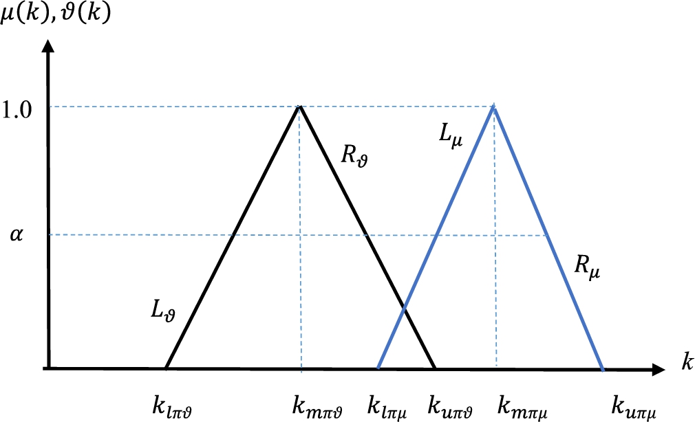
infor550_g002.jpg
Fig. 2
$\langle \textit{around}\hspace{2.5pt}{k_{\pi \mu }},\hspace{2.5pt}\textit{around}\hspace{2.5pt}{k_{\pi \vartheta }}\rangle $.
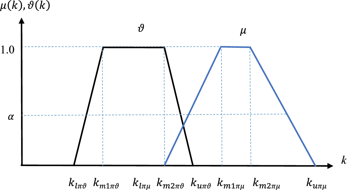
infor550_g003.jpg
Fig. 3
$\langle \textit{between}\hspace{2.5pt}{k_{m1\pi \mu }}\hspace{2.5pt}\textit{and}\hspace{2.5pt}{k_{m2\pi \mu }},\hspace{2.5pt}\textit{between}\hspace{2.5pt}{k_{m1\pi \vartheta }}\hspace{2.5pt}\textit{and}\hspace{2.5pt}{k_{m2\pi \vartheta }}\rangle $.
For triangular fuzzy proportion prediction:
(67)
\[ \langle x;{k_{\pi \mu }},{k_{\pi \vartheta }}\rangle .=\langle x;\hspace{2.5pt}\textit{around}\hspace{2.5pt}{k_{\pi \mu }},\hspace{2.5pt}\textit{around}\hspace{2.5pt}{k_{\pi \vartheta }}\rangle \]
or
(68)
\[ \langle x;{k_{\pi \mu }},{k_{\pi \vartheta }}\rangle .=\big\langle x;({k_{l\pi \mu }},{k_{m\pi \mu }},{k_{u\pi \mu }}),({k_{l\pi \vartheta }},{k_{m\pi \vartheta }},{k_{u\pi \vartheta }})\big\rangle ,\]
satisfying that $({k_{u\pi \mu }}+{k_{u\pi \vartheta }}+1)\times \pi =1$. The triangular membership function is given by Eq. (69) and Eq. (70):
(69)
\[ \mu ({k_{\pi \mu }})=\left\{\begin{array}{l@{\hskip4.0pt}l}0,\hspace{1em}& k\leqslant {k_{l\pi \mu }},\\ {} \frac{k-{k_{l\pi \mu }}}{{k_{m\pi \mu }}-{k_{l\pi \mu }}},\hspace{1em}& {k_{l\pi \mu }}\leqslant k\leqslant {k_{m\pi \mu }},\\ {} \frac{k-{k_{u\pi \mu }}}{{k_{m\pi \mu }}-{k_{u\pi \mu }}},\hspace{1em}& {k_{m\pi \mu }}\leqslant k\leqslant {k_{u\pi \mu }},\\ {} 0,\hspace{1em}& k\geqslant {k_{u\pi \mu }}\end{array}\right.\]
and
(70)
\[ \mu ({k_{\pi \vartheta }})=\left\{\begin{array}{l@{\hskip4.0pt}l}0,\hspace{1em}& k\leqslant {k_{l\pi \vartheta }},\\ {} \frac{k-{k_{l\pi \vartheta }}}{{k_{m\pi \vartheta }}-{k_{l\pi \vartheta }}},\hspace{1em}& {k_{l\pi \vartheta }}\leqslant k\leqslant {k_{m\pi \vartheta }},\\ {} \frac{k-{k_{u\pi \vartheta }}}{{k_{m\pi \vartheta }}-{k_{u\pi \vartheta }}},\hspace{1em}& {k_{m\pi \vartheta }}\leqslant k\leqslant {k_{u\pi \vartheta }},\\ {} 0,\hspace{1em}& k\geqslant {k_{u\pi \vartheta }}.\end{array}\right.\]
And for trapezoidal fuzzy proportion prediction:
(71)
\[ \langle x;{k_{\pi \mu }},{k_{\pi \vartheta }}\rangle .=\langle x;\hspace{2.5pt}\textit{between}\hspace{2.5pt}{k_{m1\pi \mu }}\hspace{2.5pt}\textit{and}\hspace{2.5pt}{k_{m2\pi \mu }},\hspace{2.5pt}\textit{between}\hspace{2.5pt}{k_{m1\pi \vartheta }}\hspace{2.5pt}\textit{and}\hspace{2.5pt}{k_{m2\pi \vartheta }}\rangle \]
or
(72)
\[ \langle x;{k_{\pi \mu }},{k_{\pi \vartheta }}\rangle .=\big\langle x;({k_{l\pi \mu }},{k_{m1\pi \mu }},{k_{m2\pi \mu }},{k_{u\pi \mu }}),({k_{l\pi \vartheta }},{k_{m1\pi \vartheta }},{k_{m2\pi \vartheta }},{k_{u\pi \vartheta }})\big\rangle ,\]
satisfying that $({k_{u\pi \mu }}+{k_{u\pi \vartheta }}+1)\times \pi =1$. The trapezoidal membership function is given by Eq. (73) and Eq. (74):
(73)
\[ \mu ({k_{\pi \mu }})=\left\{\begin{array}{l@{\hskip4.0pt}l}0,\hspace{1em}& k\leqslant {k_{l\pi \mu }},\\ {} \frac{k-{k_{l\pi \mu }}}{{k_{m1\pi \mu }}-{k_{l\pi \mu }}},\hspace{1em}& {k_{l\pi \mu }}\leqslant k\leqslant {k_{m1\pi \mu }},\\ {} 1,\hspace{1em}& {k_{m1\pi \mu }}\leqslant k\leqslant {k_{m2\pi \mu }},\\ {} \frac{k-{k_{u\pi \mu }}}{{k_{m2\pi \mu }}-{k_{u\pi \mu }}},\hspace{1em}& {k_{m2\pi \mu }}\leqslant k\leqslant {k_{u\pi \mu }},\\ {} 0,\hspace{1em}& k\geqslant {k_{u\pi \mu }}\end{array}\right.\]
and
(74)
\[ \mu ({k_{\pi \vartheta }})=\left\{\begin{array}{l@{\hskip4.0pt}l}0,\hspace{1em}& k\leqslant {k_{l\pi \vartheta }},\\ {} \frac{k-{k_{l\pi \vartheta }}}{{k_{m1\pi \vartheta }}-{k_{l\pi \vartheta }}},\hspace{1em}& {k_{l\pi \vartheta }}\leqslant k\leqslant {k_{m1\pi \vartheta }},\\ {} 1,\hspace{1em}& {k_{m1\pi \vartheta }}\leqslant k\leqslant {k_{m2\pi \vartheta }},\\ {} \frac{k-{k_{u\pi \vartheta }}}{{k_{m2\pi \vartheta }}-{k_{u\pi \vartheta }}},\hspace{1em}& {k_{m2\pi \vartheta }}\leqslant k\leqslant {k_{u\pi \vartheta }},\\ {} 0,\hspace{1em}& k\geqslant {k_{u\pi \vartheta }}.\end{array}\right.\]
We obtain the corresponding α – cut multiplication by a constant and α – cut power operations in the following. Based on the triangular membership functions of proportions and their α – cuts, Eq. (5) becomes equal to Eq. (75).
(75)
\[ {\tilde{A}_{\alpha }}=\left\{\hspace{-0.1667em}\begin{array}{l}\left[\hspace{-0.1667em}\begin{array}{l}(({k_{m\pi \mu }}-{k_{l\pi \mu }})\alpha +{k_{l\pi \mu }})\frac{1}{1+(({k_{m\pi \mu }}-{k_{l\pi \mu }})\alpha +{k_{l\pi \mu }})+(({k_{m\pi \vartheta }}-{k_{u\pi \vartheta }})\alpha +{k_{u\pi \vartheta }})},\\ {} (({k_{m\pi \mu }}-{k_{u\pi \mu }})\alpha +{k_{u\pi \mu }})\frac{1}{1+(({k_{m\pi \mu }}-{k_{u\pi \mu }})\alpha +{k_{u\pi \mu }})+(({k_{m\pi \vartheta }}-{k_{u\pi \vartheta }})\alpha +{k_{u\pi \vartheta }})}\end{array}\hspace{-0.1667em}\right],\\ {} \left[\hspace{-0.1667em}\begin{array}{l}(({k_{m\pi \vartheta }}-{k_{l\pi \vartheta }})\alpha +{k_{l\pi \vartheta }})\frac{1}{1+(({k_{m\pi \mu }}-{k_{l\pi \mu }})\alpha +{k_{l\pi \mu }})+(({k_{m\pi \vartheta }}-{k_{l\pi \vartheta }})\alpha +{k_{l\pi \vartheta }})},\\ {} (({k_{m\pi \vartheta }}-{k_{u\pi \vartheta }})\alpha +{k_{u\pi \vartheta }})\frac{1}{1+(({k_{m\pi \mu }}-{k_{l\pi \mu }})\alpha +{k_{l\pi \mu }})+(({k_{m\pi \vartheta }}-{k_{u\pi \vartheta }})\alpha +{k_{u\pi \vartheta }})}\end{array}\hspace{-0.1667em}\right]\end{array}\hspace{-0.1667em}\right\},\]
where the hesitancy degree is
\[\begin{aligned}{}& \bigg[\frac{1}{1+(({k_{m\pi \mu }}-{k_{u\pi \mu }})\alpha +{k_{u\pi \mu }})+(({k_{m\pi \vartheta }}-{k_{u\pi \vartheta }})\alpha +{k_{u\pi \vartheta }})},\\ {} & \hspace{1em}\frac{1}{1+(({k_{m\pi \mu }}-{k_{l\pi \mu }})\alpha +{k_{l\pi \mu }})+(({k_{m\pi \vartheta }}-{k_{l\pi \vartheta }})\alpha +{k_{l\pi \vartheta }})}\bigg].\end{aligned}\]
And Eq. (9) becomes
(76)
\[\begin{aligned}{}& \lambda \cdot {\tilde{A}_{\alpha }}\\ {} & \hspace{1em}=\left\{\hspace{-0.1667em}\begin{array}{l}\left[\hspace{-0.1667em}\begin{array}{l}1-{\big(1-(({k_{m\pi \mu }}-{k_{l\pi \mu }})\alpha +{k_{l\pi \mu }})\frac{1}{1+(({k_{m\pi \mu }}-{k_{l\pi \mu }})\alpha +{k_{l\pi \mu }})+(({k_{m\pi \vartheta }}-{k_{u\pi \vartheta }})\alpha +{k_{u\pi \vartheta }})}\big)^{\lambda }},\\ {} 1-{\big(1-(({k_{m\pi \mu }}-{k_{u\pi \mu }})\alpha +{k_{u\pi \mu }})\frac{1}{1+(({k_{m\pi \mu }}-{k_{u\pi \mu }})\alpha +{k_{u\pi \mu }})+(({k_{m\pi \vartheta }}-{k_{u\pi \vartheta }})\alpha +{k_{u\pi \vartheta }})}\big)^{\lambda }}\end{array}\hspace{-0.1667em}\right],\\ {} \left[\hspace{-0.1667em}\begin{array}{l}{\big((({k_{m\pi \vartheta }}-{k_{l\pi \vartheta }})\alpha +{k_{l\pi \vartheta }})\frac{1}{1+(({k_{m\pi \mu }}-{k_{l\pi \mu }})\alpha +{k_{l\pi \mu }})+(({k_{m\pi \vartheta }}-{k_{l\pi \vartheta }})\alpha +{k_{l\pi \vartheta }})}\big)^{\lambda }},\\ {} {\big((({k_{m\pi \vartheta }}-{k_{u\pi \vartheta }})\alpha +{k_{u\pi \vartheta }})\frac{1}{1+(({k_{m\pi \mu }}-{k_{l\pi \mu }})\alpha +{k_{l\pi \mu }})+(({k_{m\pi \vartheta }}-{k_{u\pi \vartheta }})\alpha +{k_{u\pi \vartheta }})}\big)^{\lambda }}\end{array}\hspace{-0.1667em}\right]\end{array}\hspace{-0.1667em}\right\},\end{aligned}\]
where the hesitancy degree is
\[\begin{aligned}{}& \bigg[{\bigg(\frac{1}{1+(({k_{m\pi \mu }}-{k_{u\pi \mu }})\alpha +{k_{u\pi \mu }})+(({k_{m\pi \vartheta }}-{k_{u\pi \vartheta }})\alpha +{k_{u\pi \vartheta }})}\bigg)^{\lambda }},\\ {} & \hspace{1em}{\bigg(\frac{1}{1+(({k_{m\pi \mu }}-{k_{l\pi \mu }})\alpha +{k_{l\pi \mu }})+(({k_{m\pi \vartheta }}-{k_{l\pi \vartheta }})\alpha +{k_{l\pi \vartheta }})}\bigg)^{\lambda }}\bigg].\end{aligned}\]
And Eq. (10) becomes
(77)
\[\begin{aligned}{}{\tilde{A}_{\alpha }^{\lambda }}& =\left\{\left[\hspace{-0.1667em}\begin{array}{l}{\big((({k_{m\pi \mu }}-{k_{l\pi \mu }})\alpha +{k_{l\pi \mu }})\frac{1}{1+(({k_{m\pi \mu }}-{k_{l\pi \mu }})\alpha +{k_{l\pi \mu }})+(({k_{m\pi \vartheta }}-{k_{u\pi \vartheta }})\alpha +{k_{u\pi \vartheta }})}\big)^{\lambda }},\\ {} {\big((({k_{m\pi \mu }}-{k_{u\pi \mu }})\alpha +{k_{u\pi \mu }})\frac{1}{1+(({k_{m\pi \mu }}-{k_{u\pi \mu }})\alpha +{k_{u\pi \mu }})+(({k_{m\pi \vartheta }}-{k_{l\pi \vartheta }})\alpha +{k_{l\pi \vartheta }})}\big)^{\lambda }}\end{array}\hspace{-0.1667em}\right]\right.,\\ {} & \hspace{1em}\left.\left[\hspace{-0.1667em}\begin{array}{l}1-{\big(1-(({k_{m\pi \vartheta }}-{k_{l\pi \vartheta }})\alpha +{k_{l\pi \vartheta }})\frac{1}{1+(({k_{m\pi \mu }}-{k_{u\pi \mu }})\alpha +{k_{u\pi \mu }})+(({k_{m\pi \vartheta }}-{k_{l\pi \vartheta }})\alpha +{k_{l\pi \vartheta }})}\big)^{\lambda }},\\ {} 1-{\big(1-(({k_{m\pi \vartheta }}-{k_{u\pi \vartheta }})\alpha +{k_{u\pi \vartheta }})\frac{1}{1+(({k_{m\pi \mu }}-{k_{l\pi \mu }})\alpha +{k_{l\pi \mu }})+(({k_{m\pi \vartheta }}-{k_{u\pi \vartheta }})\alpha +{k_{u\pi \vartheta }})}\big)^{\lambda }}\end{array}\hspace{-0.1667em}\right]\hspace{-0.1667em}\right\},\end{aligned}\]
where the hesitancy degree is
\[\begin{aligned}{}& \bigg[1-{(1-\frac{1}{1+(({k_{m\pi \mu }}-{k_{u\pi \mu }})\alpha +{k_{u\pi \mu }})+(({k_{m\pi \vartheta }}-{k_{u\pi \vartheta }})\alpha +{k_{u\pi \vartheta }})})^{\lambda }},\\ {} & \hspace{1em}1-{(1-\frac{1}{1+(({k_{m\pi \mu }}-{k_{l\pi \mu }})\alpha +{k_{l\pi \mu }})+(({k_{m\pi \vartheta }}-{k_{l\pi \vartheta }})\alpha +{k_{l\pi \vartheta }})})^{\lambda }}\bigg].\end{aligned}\]

3.2 Imprecise Proportional Pythagorean Fuzzy Sets (PPyFS)

When PPyFS are considered, Figs. 4 and 5 are replaced by Figs. 2 and 3, respectively, which present larger values of membership and non-membership degrees.
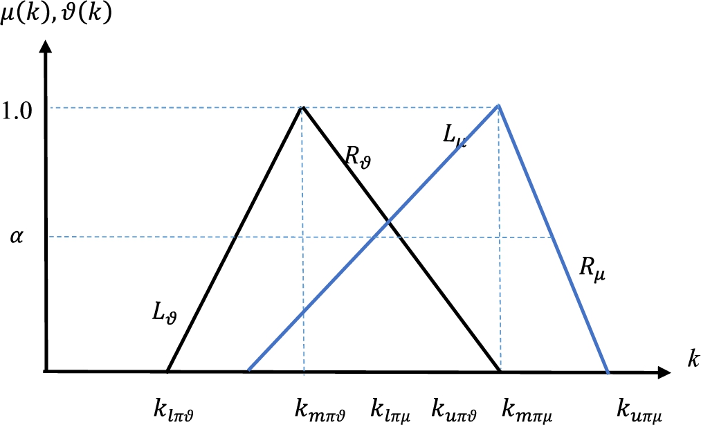
infor550_g004.jpg
Fig. 4
$\langle \textit{around}\hspace{2.5pt}{k_{\pi \mu }},\hspace{2.5pt}\textit{around}\hspace{2.5pt}{k_{\pi \vartheta }}\rangle $.
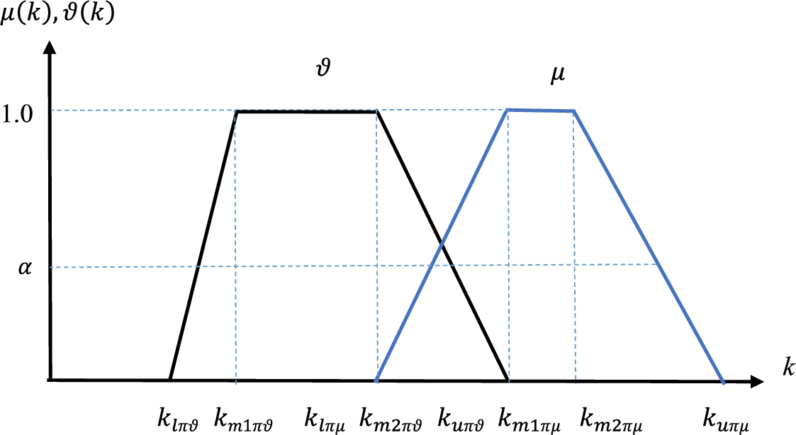
infor550_g005.jpg
Fig. 5
$\langle \textit{between}\hspace{2.5pt}{k_{m1\pi \mu }}\hspace{2.5pt}\textit{and}\hspace{2.5pt}{k_{m2\pi \mu }},\hspace{2.5pt}\textit{between}\hspace{2.5pt}{k_{m1\pi \vartheta }}\hspace{2.5pt}\textit{and}\hspace{2.5pt}{k_{m2\pi \vartheta }}\rangle $.
Using triangular $\alpha -\textit{cut}$ in Fig. 4, an imprecise PPyFS can be given as in Eq. (78).
(78)
\[ {\tilde{A}_{\alpha }}=\left\{\hspace{-0.1667em}\begin{array}{l}\left[\hspace{-0.1667em}\hspace{-0.1667em}\begin{array}{l}(({k_{m\pi \mu }}-{k_{l\pi \mu }})\alpha +{k_{l\pi \mu }})\sqrt{\frac{1}{1+{(({k_{m\pi \mu }}-{k_{l\pi \mu }})\alpha +{k_{l\pi \mu }})^{2}}+{(({k_{m\pi \vartheta }}-{k_{u\pi \vartheta }})\alpha +{k_{u\pi \vartheta }})^{2}}}},\\ {} (({k_{m\pi \mu }}-{k_{u\pi \mu }})\alpha +{k_{u\pi \mu }})\sqrt{\frac{1}{1+{(({k_{m\pi \mu }}-{k_{u\pi \mu }})\alpha +{k_{u\pi \mu }})^{2}}+{(({k_{m\pi \vartheta }}-{k_{l\pi \vartheta }})\alpha +{k_{l\pi \vartheta }})^{2}}}}\end{array}\right],\\ {} \left[\hspace{-0.1667em}\hspace{-0.1667em}\begin{array}{l}(({k_{m\pi \vartheta }}-{k_{l\pi \vartheta }})\alpha +{k_{l\pi \vartheta }})\sqrt{\frac{1}{1+{(({k_{m\pi \mu }}-{k_{u\pi \mu }})\alpha +{k_{u\pi \mu }})^{2}}+{(({k_{m\pi \vartheta }}-{k_{l\pi \vartheta }})\alpha +{k_{l\pi \vartheta }})^{2}}}},\\ {} (({k_{m\pi \vartheta }}-{k_{u\pi \vartheta }})\alpha +{k_{u\pi \vartheta }})\sqrt{\frac{1}{1+{(({k_{m\pi \mu }}-{k_{l\pi \mu }})\alpha +{k_{l\pi \mu }})^{2}}+{(({k_{m\pi \vartheta }}-{k_{u\pi \vartheta }})\alpha +{k_{u\pi \vartheta }})^{2}}}}\end{array}\hspace{-0.1667em}\right]\end{array}\hspace{-0.1667em}\right\}\]
with the hesitancy degree of
\[\begin{aligned}{}& \left[\sqrt{\frac{1}{1+{(({k_{m\pi \mu }}-{k_{u\pi \mu }})\alpha +{k_{u\pi \mu }})^{2}}+{(({k_{m\pi \vartheta }}-{k_{u\pi \vartheta }})\alpha +{k_{u\pi \vartheta }})^{2}}}},\right.\\ {} & \hspace{1em}\left.\sqrt{\frac{1}{1+{(({k_{m\pi \mu }}-{k_{l\pi \mu }})\alpha +{k_{l\pi \mu }})^{2}}+{(({k_{m\pi \vartheta }}-{k_{l\pi \vartheta }})\alpha +{k_{l\pi \vartheta }})^{2}}}}\hspace{0.1667em}\right].\end{aligned}\]
And Eq. (9) becomes
(79)
\[\begin{aligned}{}& \lambda \cdot {\tilde{A}_{\alpha }}\\ {} & \hspace{1em}=\left\{\hspace{-0.1667em}\begin{array}{l}\left[\hspace{-0.1667em}\hspace{-0.1667em}\begin{array}{l}1-{\big(1-(({k_{m\pi \mu }}-{k_{l\pi \mu }})\alpha +{k_{l\pi \mu }})\sqrt{\frac{1}{1+{(({k_{m\pi \mu }}-{k_{l\pi \mu }})\alpha +{k_{l\pi \mu }})^{2}}+{(({k_{m\pi \vartheta }}-{k_{u\pi \vartheta }})\alpha +{k_{u\pi \vartheta }})^{2}}}}\big)^{\lambda }},\\ {} 1-{\big(1-(({k_{m\pi \mu }}-{k_{u\pi \mu }})\alpha +{k_{u\pi \mu }})\sqrt{\frac{1}{1+{(({k_{m\pi \mu }}-{k_{u\pi \mu }})\alpha +{k_{u\pi \mu }})^{2}}+{(({k_{m\pi \vartheta }}-{k_{l\pi \vartheta }})\alpha +{k_{l\pi \vartheta }})^{2}}}}\big)^{\lambda }}\end{array}\hspace{-0.1667em}\hspace{-0.1667em}\right],\\ {} \left[\hspace{-0.1667em}\hspace{-0.1667em}\begin{array}{l}{\big((({k_{m\pi \vartheta }}-{k_{l\pi \vartheta }})\alpha +{k_{l\pi \vartheta }})\sqrt{\frac{1}{1+{(({k_{m\pi \mu }}-{k_{u\pi \mu }})\alpha +{k_{u\pi \mu }})^{2}}+{(({k_{m\pi \vartheta }}-{k_{l\pi \vartheta }})\alpha +{k_{l\pi \vartheta }})^{2}}}}\big)^{\lambda }},\\ {} {\big((({k_{m\pi \vartheta }}-{k_{u\pi \vartheta }})\alpha +{k_{u\pi \vartheta }})\sqrt{\frac{1}{1+{(({k_{m\pi \mu }}-{k_{l\pi \mu }})\alpha +{k_{l\pi \mu }})^{2}}+{(({k_{m\pi \vartheta }}-{k_{u\pi \vartheta }})\alpha +{k_{u\pi \vartheta }})^{2}}}}\big)^{\lambda }}\end{array}\hspace{-0.1667em}\hspace{-0.1667em}\right]\end{array}\hspace{-0.1667em}\hspace{-0.1667em}\right\},\end{aligned}\]
where the hesitancy degree is
\[\begin{aligned}{}& \left[{\bigg(\sqrt{\frac{1}{1+{(({k_{m\pi \mu }}-{k_{u\pi \mu }})\alpha +{k_{u\pi \mu }})^{2}}+{(({k_{m\pi \vartheta }}-{k_{u\pi \vartheta }})\alpha +{k_{u\pi \vartheta }})^{2}}}}\bigg)^{\lambda }},\right.\\ {} & \hspace{1em}\left.{\bigg(\sqrt{\frac{1}{1+{(({k_{m\pi \mu }}-{k_{l\pi \mu }})\alpha +{k_{l\pi \mu }})^{2}}+{(({k_{m\pi \vartheta }}-{k_{l\pi \vartheta }})\alpha +{k_{l\pi \vartheta }})^{2}}}}\bigg)^{\lambda }}\right].\end{aligned}\]
And Eq. (10) becomes
(80)
\[\begin{aligned}{}{\tilde{A}_{\alpha }^{\lambda }}& =\left\{\left[\hspace{-0.1667em}\hspace{-0.1667em}\begin{array}{l}{\big((({k_{m\pi \mu }}-{k_{l\pi \mu }})\alpha +{k_{l\pi \mu }})\sqrt{\frac{1}{1+{(({k_{m\pi \mu }}-{k_{l\pi \mu }})\alpha +{k_{l\pi \mu }})^{2}}+{(({k_{m\pi \vartheta }}-{k_{u\pi \vartheta }})\alpha +{k_{u\pi \vartheta }})^{2}}}}\hspace{0.1667em}\big)^{\lambda }},\\ {} {\big((({k_{m\pi \mu }}-{k_{u\pi \mu }})\alpha +{k_{u\pi \mu }})\sqrt{\frac{1}{1+{(({k_{m\pi \mu }}-{k_{u\pi \mu }})\alpha +{k_{u\pi \mu }})^{2}}+{(({k_{m\pi \vartheta }}-{k_{l\pi \vartheta }})\alpha +{k_{l\pi \vartheta }})^{2}}}}\hspace{0.1667em}\big)^{\lambda }}\end{array}\hspace{-0.1667em}\hspace{-0.1667em}\right]\right.,\\ {} & \hspace{1em}\left.\left[\hspace{-0.1667em}\hspace{-0.1667em}\begin{array}{l}1-{\big(1-(({k_{m\pi \vartheta }}-{k_{l\pi \vartheta }})\alpha +{k_{l\pi \vartheta }})\sqrt{\frac{1}{1+{(({k_{m\pi \mu }}-{k_{u\pi \mu }})\alpha +{k_{u\pi \mu }})^{2}}+{(({k_{m\pi \vartheta }}-{k_{l\pi \vartheta }})\alpha +{k_{l\pi \vartheta }})^{2}}}}\hspace{0.1667em}\big)^{\lambda }},\\ {} 1-{\big(1-(({k_{m\pi \vartheta }}-{k_{u\pi \vartheta }})\alpha +{k_{u\pi \vartheta }})\sqrt{\frac{1}{1+{(({k_{m\pi \mu }}-{k_{l\pi \mu }})\alpha +{k_{l\pi \mu }})^{2}}+{(({k_{m\pi \vartheta }}-{k_{u\pi \vartheta }})\alpha +{k_{u\pi \vartheta }})^{2}}}}\hspace{0.1667em}\big)^{\lambda }}\end{array}\hspace{-0.1667em}\hspace{-0.1667em}\right]\right\},\end{aligned}\]
where the hesitancy degree is
\[\begin{array}{r}\displaystyle \left[1-{\bigg(1-\sqrt{\frac{1}{1+{(({k_{m\pi \mu }}-{k_{u\pi \mu }})\alpha +{k_{u\pi \mu }})^{2}}+{(({k_{m\pi \vartheta }}-{k_{u\pi \vartheta }})\alpha +{k_{u\pi \vartheta }})^{2}}}}\hspace{0.1667em}\bigg)^{\lambda }},\right.\\ {} \displaystyle \left.1-{\bigg(1-\sqrt{\frac{1}{1+{(({k_{m\pi \mu }}-{k_{l\pi \mu }})\alpha +{k_{l\pi \mu }})^{2}}+{(({k_{m\pi \vartheta }}-{k_{l\pi \vartheta }})\alpha +{k_{l\pi \vartheta }})^{2}}}}\hspace{0.1667em}\bigg)^{\lambda }}\right].\end{array}\]

3.3 Imprecise Proportional Picture Fuzzy Sets (PPiFS)

Using triangular $\alpha -\textit{cut}$, an imprecise PPiFS can be given as in Eq. (79). Figure 6 illustrates the triangular continuous functions of the imprecise membership, non-membership, and hesitancy parameters.
(81)
\[ {\tilde{A}_{\alpha }}=\left\{\hspace{-0.1667em}\hspace{-0.1667em}\begin{array}{l}\left[\begin{array}{l}(({k_{m\pi \mu }}-{k_{l\pi \mu }})\alpha +{k_{l\pi \mu }})\frac{1}{1+(({k_{m\pi \mu }}-{k_{l\pi \mu }})\alpha +{k_{l\pi \mu }})+(({k_{m\pi \vartheta }}-{k_{u\pi \vartheta }})\alpha +{k_{u\pi \vartheta }})},\\ {} (({k_{m\pi \mu }}-{k_{u\pi \mu }})\alpha +{k_{u\pi \mu }})\frac{1}{1+(({k_{m\pi \mu }}-{k_{u\pi \mu }})\alpha +{k_{u\pi \mu }})+(({k_{m\pi \vartheta }}-{k_{u\pi \vartheta }})\alpha +{k_{u\pi \vartheta }})}\end{array}\right],\\ {} \left[\begin{array}{l}\frac{1}{1+(({k_{m\pi \mu }}-{k_{u\pi \mu }})\alpha +{k_{u\pi \mu }})+(({k_{m\pi \vartheta }}-{k_{u\pi \vartheta }})\alpha +{k_{u\pi \vartheta }})},\\ {} \frac{1}{1+(({k_{m\pi \mu }}-{k_{l\pi \mu }})\alpha +{k_{l\pi \mu }})+(({k_{m\pi \vartheta }}-{k_{l\pi \vartheta }})\alpha +{k_{l\pi \vartheta }})}\end{array}\right],\\ {} \left[\begin{array}{l}(({k_{m\pi \vartheta }}-{k_{l\pi \vartheta }})\alpha +{k_{l\pi \vartheta }})\frac{1}{1+(({k_{m\pi \mu }}-{k_{l\pi \mu }})\alpha +{k_{l\pi \mu }})+(({k_{m\pi \vartheta }}-{k_{l\pi \vartheta }})\alpha +{k_{l\pi \vartheta }})},\\ {} (({k_{m\pi \vartheta }}-{k_{u\pi \vartheta }})\alpha +{k_{u\pi \vartheta }})\frac{1}{1+(({k_{m\pi \mu }}-{k_{l\pi \mu }})\alpha +{k_{l\pi \mu }})+(({k_{m\pi \vartheta }}-{k_{u\pi \vartheta }})\alpha +{k_{u\pi \vartheta }})}\end{array}\right]\end{array}\hspace{-0.1667em}\right\}.\]
And Eq. (9) becomes
(82)
\[ \lambda \cdot {\tilde{A}_{\alpha }}=\left\{\hspace{-0.1667em}\hspace{-0.1667em}\begin{array}{l}\left[\begin{array}{l}1-{\big(1-(({k_{m\pi \mu }}-{k_{l\pi \mu }})\alpha +{k_{l\pi \mu }})\frac{1}{1+(({k_{m\pi \mu }}-{k_{l\pi \mu }})\alpha +{k_{l\pi \mu }})+(({k_{m\pi \vartheta }}-{k_{u\pi \vartheta }})\alpha +{k_{u\pi \vartheta }})}\big)^{\lambda }},\\ {} 1-{\big(1-(({k_{m\pi \mu }}-{k_{u\pi \mu }})\alpha +{k_{u\pi \mu }})\frac{1}{1+(({k_{m\pi \mu }}-{k_{u\pi \mu }})\alpha +{k_{u\pi \mu }})+(({k_{m\pi \vartheta }}-{k_{u\pi \vartheta }})\alpha +{k_{u\pi \vartheta }})}\big)^{\lambda }}\end{array}\hspace{-0.1667em}\right],\\ {} \left[\begin{array}{l}{\big(\frac{1}{1+(({k_{m\pi \mu }}-{k_{u\pi \mu }})\alpha +{k_{u\pi \mu }})+(({k_{m\pi \vartheta }}-{k_{u\pi \vartheta }})\alpha +{k_{u\pi \vartheta }})}\big)^{\lambda }},\\ {} {\big(\frac{1}{1+(({k_{m\pi \mu }}-{k_{l\pi \mu }})\alpha +{k_{l\pi \mu }})+(({k_{m\pi \vartheta }}-{k_{l\pi \vartheta }})\alpha +{k_{l\pi \vartheta }})}\big)^{\lambda }}\end{array}\right],\\ {} \left[\begin{array}{l}{\big((({k_{m\pi \vartheta }}-{k_{l\pi \vartheta }})\alpha +{k_{l\pi \vartheta }})\frac{1}{1+(({k_{m\pi \mu }}-{k_{l\pi \mu }})\alpha +{k_{l\pi \mu }})+(({k_{m\pi \vartheta }}-{k_{l\pi \vartheta }})\alpha +{k_{l\pi \vartheta }})}\big)^{\lambda }},\\ {} {\big((({k_{m\pi \vartheta }}-{k_{u\pi \vartheta }})\alpha +{k_{u\pi \vartheta }})\frac{1}{1+(({k_{m\pi \mu }}-{k_{l\pi \mu }})\alpha +{k_{l\pi \mu }})+(({k_{m\pi \vartheta }}-{k_{u\pi \vartheta }})\alpha +{k_{u\pi \vartheta }})}\big)^{\lambda }}\end{array}\hspace{-0.1667em}\right]\end{array}\hspace{-0.1667em}\right\}.\]
And Eq. (10) becomes
(83)
\[\begin{aligned}{}{\tilde{A}_{\alpha }^{\lambda }}& =\left\{\left[\begin{array}{l}{\big((({k_{m\pi \mu }}-{k_{l\pi \mu }})\alpha +{k_{l\pi \mu }})\frac{1}{1+(({k_{m\pi \mu }}-{k_{l\pi \mu }})\alpha +{k_{l\pi \mu }})+(({k_{m\pi \vartheta }}-{k_{u\pi \vartheta }})\alpha +{k_{u\pi \vartheta }})}\big)^{\lambda }},\\ {} {\big((({k_{m\pi \mu }}-{k_{u\pi \mu }})\alpha +{k_{u\pi \mu }})\frac{1}{1+(({k_{m\pi \mu }}-{k_{u\pi \mu }})\alpha +{k_{u\pi \mu }})+(({k_{m\pi \vartheta }}-{k_{l\pi \vartheta }})\alpha +{k_{l\pi \vartheta }})}\big)^{\lambda }}\end{array}\hspace{-0.1667em}\right]\right.,\\ {} & \hspace{1em}\left[\hspace{-0.1667em}\begin{array}{l}1-{\big(1-\frac{1}{1+(({k_{m\pi }}-{k_{u\pi }})\alpha +{k_{u\pi }})+(({k_{m\pi }}-{k_{u\pi }})\alpha +{k_{u\pi }})}\big)^{\lambda }},\\ {} 1-{\big(1-\frac{1}{1+(({k_{m\pi }}-{k_{l\pi }})\alpha +{k_{l\pi }})+(({k_{m\pi }}-{k_{l\pi }})\alpha +{k_{l\pi }})}\big)^{\lambda }}\end{array}\hspace{-0.1667em}\right],\\ {} & \hspace{1em}\left.\left[\begin{array}{l}1-{\big(1-(({k_{m\pi \vartheta }}-{k_{l\pi \vartheta }})\alpha +{k_{l\pi \vartheta }})\frac{1}{1+(({k_{m\pi \mu }}-{k_{u\pi \mu }})\alpha +{k_{u\pi \mu }})+(({k_{m\pi \vartheta }}-{k_{l\pi \vartheta }})\alpha +{k_{l\pi \vartheta }})}\big)^{\lambda }},\\ {} 1-{\big(1-(({k_{m\pi \vartheta }}-{k_{u\pi \vartheta }})\alpha +{k_{u\pi \vartheta }})\frac{1}{1+(({k_{m\pi \mu }}-{k_{l\pi \mu }})\alpha +{k_{l\pi \mu }})+(({k_{m\pi \vartheta }}-{k_{u\pi \vartheta }})\alpha +{k_{u\pi \vartheta }})}\big)^{\lambda }}\end{array}\hspace{-0.1667em}\right]\right\}.\end{aligned}\]
infor550_g006.jpg
Fig. 6
$\langle \textit{around}\hspace{2.5pt}{k_{\pi \mu }},\hspace{2.5pt}\textit{around}\hspace{2.5pt}{k_{\pi }},\textit{around}\hspace{2.5pt}{k_{\pi \vartheta }}\rangle $.
Figure 7 illustrates the trapezoidal continuous functions of the imprecise membership, non-membership, and hesitancy parameters.
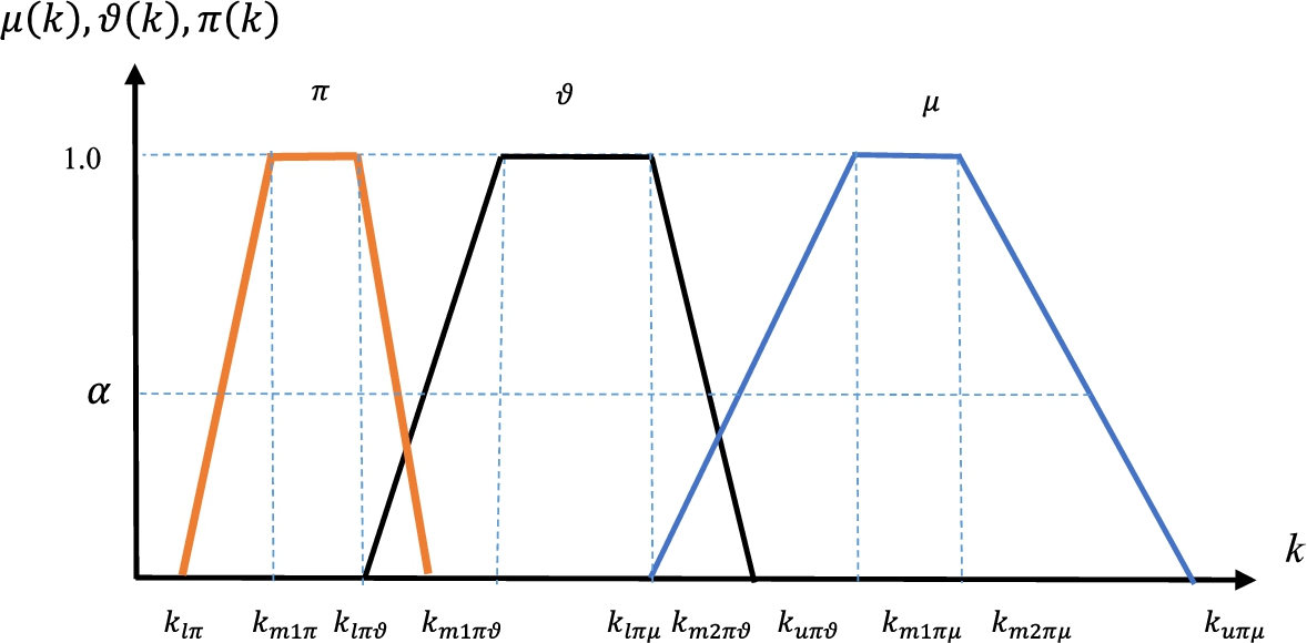
infor550_g007.jpg
Fig. 7
$\langle \textit{between}\hspace{2.5pt}{k_{m1\pi \mu }}\hspace{2.5pt}\textit{and}\hspace{2.5pt}{k_{m2\pi \mu }},\hspace{2.5pt}\textit{between}\hspace{2.5pt}{k_{m1\pi }}\hspace{2.5pt}\textit{and}\hspace{2.5pt}{k_{m2\pi ,}}\textit{between}\hspace{2.5pt}{k_{m1\pi \vartheta }}\hspace{2.5pt}\textit{and}\hspace{2.5pt}{k_{m2\pi \vartheta }}\rangle $.

3.4 Imprecise Proportional Spherical Fuzzy Sets (PSFS)

When PSFS are considered, Fig. 6 is replaced by Fig. 8, which presents larger values of membership, non-membership degrees, and hesitancy.
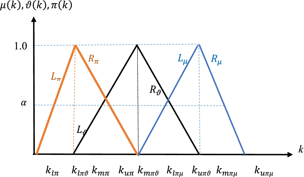
infor550_g008.jpg
Fig. 8
$\langle \textit{around}\hspace{2.5pt}{k_{\pi \mu }},\hspace{2.5pt}\textit{around}\hspace{2.5pt}{k_{\pi }},\hspace{2.5pt}\textit{around}\hspace{2.5pt}{k_{\pi \vartheta }}\rangle $.
Using triangular $\alpha -\textit{cut}$, an imprecise PSFS can be given as Eq. (84).
(84)
\[ {\tilde{A}_{\alpha }}=\left\{\begin{array}{l}\left[\begin{array}{l}(({k_{m\pi \mu }}-{k_{l\pi \mu }})\alpha +{k_{l\pi \mu }})\sqrt{\frac{1}{1+{(({k_{m\pi \mu }}-{k_{l\pi \mu }})\alpha +{k_{l\pi \mu }})^{2}}+{(({k_{m\pi \vartheta }}-{k_{u\pi \vartheta }})\alpha +{k_{u\pi \vartheta }})^{2}}}},\\ {} (({k_{m\pi \mu }}-{k_{u\pi \mu }})\alpha +{k_{u\pi \mu }})\sqrt{\frac{1}{1+{(({k_{m\pi \mu }}-{k_{u\pi \mu }})\alpha +{k_{u\pi \mu }})^{2}}+{(({k_{m\pi \vartheta }}-{k_{l\pi \vartheta }})\alpha +{k_{l\pi \vartheta }})^{2}}}}\end{array}\right],\\ {} \left[\begin{array}{l}\sqrt{\frac{1}{1+{(({k_{m\pi \mu }}-{k_{u\pi \mu }})\alpha +{k_{u\pi \mu }})^{2}}+{(({k_{m\pi \vartheta }}-{k_{u\pi \vartheta }})\alpha +{k_{u\pi \vartheta }})^{2}}}},\\ {} \sqrt{\frac{1}{1+{(({k_{m\pi \mu }}-{k_{l\pi \mu }})\alpha +{k_{l\pi \mu }})^{2}}+{(({k_{m\pi \vartheta }}-{k_{l\pi \vartheta }})\alpha +{k_{l\pi \vartheta }})^{2}}}}\end{array}\right],\\ {} \left[\begin{array}{l}(({k_{m\pi \vartheta }}-{k_{l\pi \vartheta }})\alpha +{k_{l\pi \vartheta }})\sqrt{\frac{1}{1+{(({k_{m\pi \mu }}-{k_{u\pi \mu }})\alpha +{k_{u\pi \mu }})^{2}}+{(({k_{m\pi \vartheta }}-{k_{l\pi \vartheta }})\alpha +{k_{l\pi \vartheta }})^{2}}}},\\ {} (({k_{m\pi \vartheta }}-{k_{u\pi \vartheta }})\alpha +{k_{u\pi \vartheta }})\sqrt{\frac{1}{1+{(({k_{m\pi \mu }}-{k_{l\pi \mu }})\alpha +{k_{l\pi \mu }})^{2}}+{(({k_{m\pi \vartheta }}-{k_{u\pi \vartheta }})\alpha +{k_{u\pi \vartheta }})^{2}}}}\end{array}\right]\end{array}\hspace{-0.1667em}\hspace{-0.1667em}\right\}.\]
And Eq. (9) becomes
(85)
\[\begin{aligned}{}& \lambda \cdot {\tilde{A}_{\alpha }}\\ {} & \hspace{1em}=\left\{\hspace{-0.1667em}\hspace{-0.1667em}\begin{array}{l}\left[\begin{array}{l}1-{\big(1-(({k_{m\pi \mu }}-{k_{l\pi \mu }})\alpha +{k_{l\pi \mu }})\sqrt{\frac{1}{1+{(({k_{m\pi \mu }}-{k_{l\pi \mu }})\alpha +{k_{l\pi \mu }})^{2}}+{(({k_{m\pi \vartheta }}-{k_{u\pi \vartheta }})\alpha +{k_{u\pi \vartheta }})^{2}}}}\big)^{\lambda }},\\ {} 1-{\big(1-(({k_{m\pi \mu }}-{k_{u\pi \mu }})\alpha +{k_{u\pi \mu }})\sqrt{\frac{1}{1+{(({k_{m\pi \mu }}-{k_{u\pi \mu }})\alpha +{k_{u\pi \mu }})^{2}}+{(({k_{m\pi \vartheta }}-{k_{l\pi \vartheta }})\alpha +{k_{l\pi \vartheta }})^{2}}}}\big)^{\lambda }}\end{array}\hspace{-0.1667em}\right],\\ {} \left[\begin{array}{l}{\Big(\sqrt{\frac{1}{1+{(({k_{m\pi \mu }}-{k_{u\pi \mu }})\alpha +{k_{u\pi \mu }})^{2}}+{(({k_{m\pi \vartheta }}-{k_{u\pi \vartheta }})\alpha +{k_{u\pi \vartheta }})^{2}}}}\Big)^{\lambda }},\\ {} {\Big(\sqrt{\frac{1}{1+{(({k_{m\pi \mu }}-{k_{l\pi \mu }})\alpha +{k_{l\pi \mu }})^{2}}+{(({k_{m\pi \vartheta }}-{k_{l\pi \vartheta }})\alpha +{k_{l\pi \vartheta }})^{2}}}}\Big)^{\lambda }}\end{array}\right],\\ {} \left[\begin{array}{l}{\big((({k_{m\pi \vartheta }}-{k_{l\pi \vartheta }})\alpha +{k_{l\pi \vartheta }})\sqrt{\frac{1}{1+{(({k_{m\pi \mu }}-{k_{u\pi \mu }})\alpha +{k_{u\pi \mu }})^{2}}+{(({k_{m\pi \vartheta }}-{k_{l\pi \vartheta }})\alpha +{k_{l\pi \vartheta }})^{2}}}}\big)^{\lambda }},\\ {} {\big((({k_{m\pi \vartheta }}-{k_{u\pi \vartheta }})\alpha +{k_{u\pi \vartheta }})\sqrt{\frac{1}{1+{(({k_{m\pi \mu }}-{k_{l\pi \mu }})\alpha +{k_{l\pi \mu }})^{2}}+{(({k_{m\pi \vartheta }}-{k_{u\pi \vartheta }})\alpha +{k_{u\pi \vartheta }})^{2}}}}\big)^{\lambda }}\end{array}\hspace{-0.1667em}\right]\end{array}\hspace{-0.1667em}\hspace{-0.1667em}\right\}.\end{aligned}\]
And Eq. (10) becomes
(86)
\[\begin{aligned}{}{\tilde{A}_{\alpha }^{\lambda }}& =\left\{\left[\hspace{-0.1667em}\begin{array}{l}{\big((({k_{m\pi \mu }}-{k_{l\pi \mu }})\alpha +{k_{l\pi \mu }})\sqrt{\frac{1}{1+{(({k_{m\pi \mu }}-{k_{l\pi \mu }})\alpha +{k_{l\pi \mu }})^{2}}+{(({k_{m\pi \vartheta }}-{k_{u\pi \vartheta }})\alpha +{k_{u\pi \vartheta }})^{2}}}}\big)^{\lambda }},\\ {} {\big((({k_{m\pi \mu }}-{k_{u\pi \mu }})\alpha +{k_{u\pi \mu }})\sqrt{\frac{1}{1+{(({k_{m\pi \mu }}-{k_{u\pi \mu }})\alpha +{k_{u\pi \mu }})^{2}}+{(({k_{m\pi \vartheta }}-{k_{l\pi \vartheta }})\alpha +{k_{l\pi \vartheta }})^{2}}}}\big)^{\lambda }}\end{array}\hspace{-0.1667em}\hspace{-0.1667em}\right]\right.,\\ {} & \hspace{1em}\left[\hspace{-0.1667em}\begin{array}{l}1-{\big(1-\sqrt{\frac{1}{1+{(({k_{m\pi \mu }}-{k_{u\pi \mu }})\alpha +{k_{u\pi \mu }})^{2}}+{(({k_{m\pi \vartheta }}-{k_{u\pi \vartheta }})\alpha +{k_{u\pi \vartheta }})^{2}}}}\big)^{\lambda }},\\ {} 1-{\big(1-\sqrt{\frac{1}{1+{(({k_{m\pi \mu }}-{k_{l\pi \mu }})\alpha +{k_{l\pi \mu }})^{2}}+{(({k_{m\pi \vartheta }}-{k_{l\pi \vartheta }})\alpha +{k_{l\pi \vartheta }})^{2}}}}\big)^{\lambda }}\end{array}\right],\\ {} & \hspace{1em}\left.\left[\begin{array}{l}1-{\big(1-(({k_{m\pi \vartheta }}-{k_{l\pi \vartheta }})\alpha +{k_{l\pi \vartheta }})\sqrt{\frac{1}{1+{(({k_{m\pi \mu }}-{k_{u\pi \mu }})\alpha +{k_{u\pi \mu }})^{2}}+{(({k_{m\pi \vartheta }}-{k_{l\pi \vartheta }})\alpha +{k_{l\pi \vartheta }})^{2}}}}\big)^{\lambda }},\\ {} 1-{\big(1-(({k_{m\pi \vartheta }}-{k_{u\pi \vartheta }})\alpha +{k_{u\pi \vartheta }})\sqrt{\frac{1}{1+{(({k_{m\pi \mu }}-{k_{l\pi \mu }})\alpha +{k_{l\pi \mu }})^{2}}+{(({k_{m\pi \vartheta }}-{k_{u\pi \vartheta }})\alpha +{k_{u\pi \vartheta }})^{2}}}}\big)^{\lambda }}\end{array}\right]\right\}.\end{aligned}\]
Figure 7 is replaced by Fig. 9, which illustrates the trapezoidal continuous functions of the imprecise membership, non-membership, and hesitancy parameters and presents larger values of membership, non-membership degrees, and hesitancy for spherical fuzzy sets.
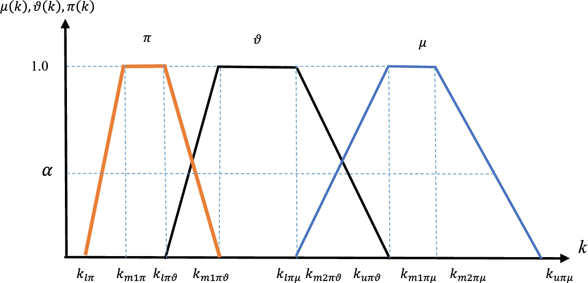
infor550_g009.jpg
Fig. 9
$\langle \textit{between}\hspace{2.5pt}{k_{m1\pi \mu }}\hspace{2.5pt}\textit{and}\hspace{2.5pt}{k_{m2\pi \mu }},\hspace{2.5pt}\textit{between}\hspace{2.5pt}{k_{m1\pi }}\hspace{2.5pt}\textit{and}\hspace{2.5pt}{k_{m2\pi ,}}\textit{between}\hspace{2.5pt}{k_{m1\pi \vartheta }}\hspace{2.5pt}\textit{and}\hspace{2.5pt}{k_{m2\pi \vartheta }}\rangle $.

4 MCDM Applications of the Proportional Fuzzy Sets

In this section, we give an MCDM application of the developed PFS extensions for both precise and imprecise definitions of proportions.
Three experts (E1, E2, and E3) evaluate four cars by considering 5 attributes, which are comfort, safety, esthetic, price, and service facilities. Each of the experts constructs his/her decision matrix as given in Table 1.
Table 1
Proportional fuzzy decision matrices of the experts.
Alternatives Comfort Safety Esthetic Price Service facilities
E-1 Criteria
Car-1 $(5,1)$ $(7,2)$ $(7,2)$ $(6,1)$ $(4,1)$
Car-2 (Around 5, Around 2) $(10,1)$ $(3,1)$ $(8,2)$ $(7,1)$
Car-3 $(5,2)$ $(6,2)$ $(4,2)$ $(6,2)$ $(6,2)$
Car-4 $(4,1)$ $(5,2)$ $(5,3)$ $(6,3)$ $(5,2)$
E-2 Criteria
Car-1 $(4,1)$ $(6,2)$ $(6,2)$ $(5,1)$ $(5,2)$
Car-2 $(7,1)$ $(8,3)$ $(4,1)$ $(7,3)$ $(6,2)$
Car-3 $(5,1)$ $(5,1)$ $(4,1)$ $(5,1)$ $(7,3)$
Car-4 $(5,1)$ $(6,2)$ $(6,2)$ $(6,2)$ (Around 6, Around 2)
E-3 Criteria
Car-1 $(5,2)$ (Around 5, Around 2) $(5,3)$ $(8,1)$ $(6,1)$
Car-2 $(4,1)$ $(7,1)$ $(5,1)$ $(7,2)$ $(4,1)$
Car-3 $(6,3)$ $(6,3)$ $(4,2)$ $(6,4)$ $(4,2)$
Car-4 $(3,1)$ $(6,1)$ $(6,3)$ $(5,3)$ $(5,2)$
Giving some values for α, we can aggregate the proportional fuzzy decision matrices. For instance, assume that the experts compromise on $\alpha =0.4$ since they are quite sure about the proportions.
When proportional intuitionistic fuzzy sets are considered, PIFWA operator in Eq. (12) gives the aggregated decision matrix in Table 2.
Table 2
PIFWA operator with proportional intuitionistic fuzzy sets.
Alternatives Comfort Safety Esthetic Price Service facilities
μ ϑ μ ϑ μ ϑ μ ϑ μ ϑ
Car-1 0.6632 0.1862 0.6026 0.6547 0.6390 0.5121 0.7545 0.1228 0.6822 0.1809
Car-2 0.6892 0.1701 0.7482 0.1511 0.6724 0.1638 0.6790 0.3540 0.6926 0.1749
Car-3 0.6606 0.2072 0.6685 0.4132 0.6173 0.3518 0.6533 0.5329 0.6215 0.4175
Car-4 0.6685 0.1657 0.6914 0.1860 0.6237 0.5467 0.6177 0.5554 0.5429 0.5217
When proportional Pythagorean fuzzy sets are considered, PPFWA operator in Eq. (26) gives the aggregated decision matrix in Table 3.
Table 3
PPFWA operator with proportional Pythagorean fuzzy sets.
Alternatives Comfort Safety Esthetic Price Service facilities
μ ϑ μ ϑ μ ϑ μ ϑ μ ϑ
Car-1 0.9390 0.2638 0.8923 0.4086 0.9185 0.3600 0.9743 0.1591 0.9471 0.2518
Car-2 0.9492 0.2336 0.9696 0.1970 0.9452 0.2306 0.9402 0.3124 0.9517 0.2411
Car-3 0.9340 0.2927 0.9382 0.2837 0.9113 0.3308 0.9284 0.3061 0.9061 0.3883
Car-4 0.9432 0.2345 0.9503 0.2562 0.9068 0.3887 0.9026 0.3967 0.8378 0.5008
When proportional picture fuzzy sets are considered, PPiFWA operator in Eq. (46) gives the aggregated decision matrix in Table 4, assuming there is no refusal degree of the judgments.
Table 4
PPFWA operator with proportional picture fuzzy sets.
Alts. Comfort Safety Esthetic Price Service facilities
μ π ϑ μ π ϑ μ π ϑ μ π ϑ μ π ϑ
Car-1 0.663 0.146 0.186 0.603 0.113 0.281 0.639 0.109 0.251 0.754 0.123 0.123 0.682 0.132 0.181
Car-2 0.689 0.131 0.170 0.748 0.092 0.151 0.672 0.164 0.164 0.679 0.094 0.226 0.693 0.128 0.175
Car-3 0.661 0.123 0.207 0.669 0.120 0.202 0.617 0.153 0.224 0.653 0.116 0.216 0.621 0.111 0.266
Car-4 0.669 0.166 0.166 0.691 0.119 0.186 0.624 0.107 0.268 0.618 0.109 0.272 0.543 0.119 0.332
Table 5
PSFWA operator with proportional spherical fuzzy sets.
Alts. Comfort Safety Esthetic Price Service facilities
μ π ϑ μ π ϑ μ π ϑ μ π ϑ μ π ϑ
Car-1 0.939 0.207 0.264 0.892 0.165 0.409 0.918 0.156 0.360 0.974 0.159 0.159 0.947 0.184 0.252
Car-2 0.949 0.180 0.234 0.970 0.120 0.197 0.945 0.231 0.231 0.940 0.130 0.312 0.952 0.176 0.241
Car-3 0.934 0.173 0.293 0.938 0.168 0.284 0.911 0.226 0.331 0.928 0.164 0.306 0.906 0.162 0.388
Car-4 0.943 0.235 0.235 0.950 0.163 0.256 0.907 0.156 0.389 0.903 0.159 0.397 0.838 0.179 0.501
When proportional spherical fuzzy sets are considered, PSFWA operator in Eq. (62) gives the aggregated decision matrix in Table 5, assuming there is no refusal degree of the judgments.
The three experts evaluate the five criteria as in Table 7 to determine their weights by considering the linguistic terms given in Table 6. Any intermediate value can be assigned if the expert is hesitant between two successive terms. For instance, if the judgment is between AA and H, then the expert can assign a PF value of $(6.5,3.5)$ or $(6,3.5)$, or $(6.5,3)$.
Table 6
Linguistic proportional fuzzy scale.
Linguistic terms (l) PF values
Certainly Low (CL) $(1,9)$
Very Low (VL) $(2,8)$
Low (L) $(3,7)$
Below Average (BA) $(4,6)$
Average (A) $(5,5)$
Above Average (AA) $(6,4)$
High (H) $(7,3)$
Very High (VH) $(8,2)$
Certainly High (CH) $(9,1)$
Table 7
Criteria evaluation by the experts.
Comfort Safety Esthetic Price Service facilities
E-1 VH VH AA CH AA
E-2 H VH H VH H
E-3 A VH BA AA VH
In the solution of the considered MCDM problem, we only use proportional intuitionistic fuzzy sets and proportional spherical fuzzy sets because of space constraints. From Table 7, the fuzzy weights are obtained by PIFWA operator using PIFS as in Table 8.
Table 8
Intuitionistic fuzzy weights based on PIFWA operator.
Comfort Safety Esthetic Price Service facilities
μ ϑ μ ϑ μ ϑ μ ϑ μ ϑ
0.6043 0.3007 0.7273 0.1818 0.5375 0.3682 0.6993 0.2017 0.6562 0.2507
Table 9
Sphericalfuzzy weights based on PSFWA operator.
Comfort Safety Esthetic Price Service facilities
μ π ϑ μ π ϑ μ π ϑ μ π ϑ μ π ϑ
0.8860 0.1315 0.4349 0.9631 0.1204 0.2408 0.8204 0.1341 0.5431 0.9490 0.1318 0.2747 0.9252 0.1280 0.3530
The weighted decision matrix using intuitionistic numbers in Table 2 and the aggregated decision matrix by PIFWA in Table 8 is given in Table 10.
Table 10
Weighted decision matrix using IFN and PIFWA.
Alternatives Comfort Safety Esthetic Price Service facilities
μ ϑ μ ϑ μ ϑ μ ϑ μ ϑ
Car-1 0.4008 0.4310 0.4383 0.7175 0.3435 0.6918 0.5276 0.2997 0.4476 0.3862
Car-2 0.4165 0.4197 0.5442 0.3054 0.3614 0.4717 0.4748 0.4843 0.4545 0.3817
Car-3 0.3992 0.4456 0.4862 0.5199 0.3318 0.5904 0.4569 0.6271 0.4078 0.5635
Car-4 0.4040 0.4166 0.5028 0.3340 0.3352 0.7136 0.4319 0.6451 0.3562 0.6416
By using intuitionistic fuzzy addition operation, we obtain the score of each alternative based on the simple additive weighting (SAW) method as in Table 11.
Table 11
IF scores based on SAW method.
IF scores Net membership $=\mu -v$ Ranking
μ v
Car-1 0.9423 0.0248 0.9176 2
Car-2 0.9513 0.0112 0.9402 1
Car-3 0.9337 0.0483 0.8853 4
Car-4 0.9280 0.0411 0.8869 3
The weighted decision matrix using spherical fuzzy numbers in Table 5 and the aggregated decision matrix by PSFWA in Table 9 is given in Table 12.
Table 12
Weighted decision matrix using SFN and PSFWA.
Alts. Comfort Safety Esthetic Price Service facilities
μ π ϑ μ π ϑ μ π ϑ μ π ϑ μ π ϑ
Car-1 0.8320 0.2397 0.4956 0.8594 0.1932 0.4639 0.7535 0.3684 0.6216 0.9247 0.2033 0.5659 0.8762 0.2110 0.4244
Car-2 0.8410 0.2183 0.4831 0.9338 0.1653 0.3075 0.7755 0.2315 0.5766 0.8923 0.1789 0.6266 0.8805 0.2054 0.4189
Car-3 0.8276 0.2118 0.5085 0.9036 0.1989 0.3658 0.7476 0.3292 0.6100 0.8810 0.2042 0.6234 0.8383 0.1908 0.5066
Car-4 0.8357 0.2635 0.4835 0.9152 0.1956 0.3462 0.7440 0.3956 0.6336 0.8566 0.1973 0.6726 0.7751 0.1992 0.5867
By using spherical fuzzy addition operation, we obtain the score of each alternative based on the simple additive weighting (SAW) method as in Table 13.
Table 13
SF scores based on SAW method.
SF scores Net membership $=\mu -\frac{\pi }{2}-v$ Ranking
μ π v
Car-1 0.9994 0.0291 0.0343 0.9505 2
Car-2 0.9997 0.0204 0.0225 0.9670 1
Car-3 0.9992 0.0329 0.0358 0.9469 3
Car-4 0.9988 0.0405 0.0418 0.9367 4
This comparative analysis based on different fuzzy set extensions’ arithmetic operations and aggregation operators gives slightly different ranking results. IF-SAW gives the ranking Car 2 > Car 1 > Car 4 > Car 3 whereas SF-SAW gives the ranking Car 2 > Car 1 > Car 3 > Car 4. This difference comes from the hesitancy computation in IFS and SFS.

5 Conclusion

We presented several proportional fuzzy set extensions including PIFS, PPyFS, PPiFS, and PSFS. The main advantage of these proportional fuzzy set extensions is their ability to determine the membership, non-membership, and hesitancy degrees easily and correctly. We developed the arithmetic operations and aggregation operators of each proportional fuzzy set extension. We also presented $\alpha -\textit{cut}$ approaches for the cases that experts are unsure to determine the proportions between the degrees. The rule is the more unsure you are, the smaller α you assign or the more sure you are, the larger α you assign. Once you determine the proportions, they are substituted into the developed equations. Then they produce the usual membership, non-membership and hesitancy degrees as in their formal definitions.
Experts cannot assign numbers with multiple decimal places for any membership degree when they directly try to assign it. The proposed proportional approaches could produce membership degrees with several decimal places. Car alternatives in the application section have been prioritized by using simple additive weighting method based on proportional intuitionistic fuzzy sets and proportional spherical fuzzy sets. A slight difference has been obtained in their rankings because of the differences in the theoretical structures of the fuzzy set extensions. Intuitionistic fuzzy sets require membership and non-membership degrees to be assigned whereas spherical fuzzy sets require hesitancy degree additionally.
The limitation of proportional fuzzy sets may be difficult to implement in cases where the degrees are independent, as in neutrosophic sets. Because in neutrosophic sets, each degree can take any value between 0 and 1, and the upper limit of the sum can be 3.
For further research, we suggest the developed proportional fuzzy sets to be employed in the extension of MCDM methods such as VIKOR, ELECTRE, WASPAS, MOORA, or COPRAS. We developed only four extensions of ordinary fuzzy sets. We developed only four proportional fuzzy extensions of ordinary fuzzy sets. The other extensions such as neutrosophic sets, fermatean fuzzy sets, q-rung orthopair fuzzy sets, or t-spherical fuzzy sets can be handled to develop their proportional fuzzy versions.

References

 
Alkan, N., Kahraman, C. (2023). Continuous intuitionistic fuzzy sets (CINFUS) and their AHP&TOPSIS extension: research proposals evaluation for grant funding. Applied Soft Computing, 145, 110579.
 
Atanassov, K. (1986). Intuitionistic fuzzy sets. Fuzzy Sets System, 20(1), 87–96.
 
Atanassov, K., Szmidt, E., Kacprzyk, J. (2010). On some ways of determining membership and non-membership functions characterizing intuitionistic fuzzy sets. In: Sixth International Workshop on IFSs, Banska Bystrica, Slovakia, 10 October 2010, pp. 26–30.
 
Atanassov, K.T. (1989). More on intuitionistic fuzzy sets. Fuzzy Sets and Systems, 33(1), 37–45.
 
Atanassov, K.T. (1999). Intuitionistic fuzzy sets. In: Intuitionistic Fuzzy Sets. Studies in Fuzziness and Soft Computing, Physica, Vol. 35, Heidelberg.
 
Atanassov, K.T. (2020). Circular intuitionistic fuzzy sets. Journal of Intelligent & Fuzzy Systems, 39(5), 5981–5986.
 
Cebi, S., Kutlu Gündoğdu, F., Kahraman, C. (2022). Operational risk analysis in business processes using decomposed fuzzy sets. Journal of Intelligent & Fuzzy Systems, 43(3), 2485–2502.
 
Chowdhury, S., Kar, R. (2020). Evaluation of approximate fuzzy membership function using linguistic input-an approached based on cubic spline. Journal of Information and Visualization, 1(2), 53–59.
 
Cuong, B.C., Kreinovich, V. (2013). Picture fuzzy sets – a new concept for computational intelligence problems. In: 2013 Third World Congress on Information and Communication Technologies (WICT 2013), Hanoi, Vietnam, 2013, pp. 1–6.
 
Dalkılıç, O. (2021). Determining the (non-)membership degrees in the range (0, 1) independently of the decision-makers for bipolar soft sets. Journal of Taibah University for Science, 15(1), 609–618.
 
Garibaldi, J.M., Ozen, T. (2007). Uncertain fuzzy reasoning: a case study in modelling expert decision making. IEEE Transactions on Fuzzy Systems, 15(1), 16–30.
 
Hasan, M.F., Sobhan, M.A. (2020). Describing fuzzy membership function and detecting the outlier by using five number summary of data. American Journal of Computational Mathematics, 10(3), 410–424. https://doi.org/10.4236/ajcm.2020.103022.
 
Jiang, L., Liao, H. (2020). Cognitive fuzzy sets for decision making. Applied Soft Computing, 93, 106374.
 
Kahraman, C., Kutlu Gündogdu, F. (2018). From 1D to 3D membership: spherical fuzzy sets. In: BOS/SOR Conference, September 24th–26th 2018, Palais Staszic. Polish Operational and Systems Research Society, Warsaw, Poland.
 
Kahraman, C. (2024). Proportional picture fuzzy sets and their AHP extension: application to waste disposal site selection. Expert Systems with Applications, 238(Part F), 122354. https://doi.org/10.1016/j.eswa.2023.122354.
 
Kutlu Gündoğdu, F., Kahraman, C. (2019). Spherical fuzzy sets and spherical fuzzy TOPSIS method. Journal of Intelligent & Fuzzy Systems, 36(1), 337–352.
 
Senapati, Y., Yager, R. (2020). Fermatean fuzzy sets. Journal of Ambient Intelligence and Humanized Computing, 11(2), 663–674.
 
Smarandache, F. (1998). Neutrosophy: Neutrosophic Probability, Set, and Logic: Analytic Synthesis & Synthetic Analysis. American Research Press.
 
Torra, V. (2010). Hesitant fuzzy sets. International Journal of Intelligent Systems, 25(6), 529–539.
 
Yager, R. (2016). Generalized orthopair fuzzy sets. IEEE Transactions on Fuzzy Systems, 25(5), 1222–1230.
 
Yager, R. (2013). Pythagorean fuzzy subsets. In: Proceedings of the 2013 Joint IFSA World Congress and NAFIPS Annual Meeting, IFSA/NAFIPS 2013, pp. 57–61. https://doi.org/10.1109/IFSA-NAFIPS.2013.6608375.
 
Yager, R.R. (1986). On the theory of bags. International Journal of General Systems, 13(1), 23–37.
 
Zadeh, L.A. (1975). The concept of a linguistic variable and its application. Information Sciences, 8(3), 199–249.

Biographies

Kahraman Cengiz
kahramanc@itu.edu.tr

C. Kahraman graduated from Kuleli Military High School in 1983. He received his BSc degree in 1988, MSc degree in 1990, and PhD degree in 1996 from industrial engineering of Istanbul Technical University. Prof. Kahraman is now a full professor at Istanbul Technical University. His research areas are engineering economics, quality control and management, statistical decision making, multicriteria decision making, and fuzzy decision making. He published about 350 journal papers and about 250 conference papers. He became a guest editor of many international journals and an editor of many international books from Springer and Atlantis Press. He is the member of editorial boards of 20 international journals. He organized various conferences such as FLINS, RACR, FSSCMIE, and INFUS. He was the vice dean of ITU Management Faculty between 2004–2007 and the head of ITU Industrial Engineering Department between 2010–2013.


Exit Reading PDF XML


Table of contents
  • 1 Introduction
  • 2 Proportional Fuzzy Sets (PIFS)
  • 3 Imprecise Proportions
  • 4 MCDM Applications of the Proportional Fuzzy Sets
  • 5 Conclusion
  • References
  • Biographies

Export citation

Copy and paste formatted citation
Placeholder

Download citation in file


Share


RSS

INFORMATICA

  • Online ISSN: 1822-8844
  • Print ISSN: 0868-4952
  • Copyright © 2023 Vilnius University

About

  • About journal

For contributors

  • OA Policy
  • Submit your article
  • Instructions for Referees
    •  

    •  

Contact us

  • Institute of Data Science and Digital Technologies
  • Vilnius University

    Akademijos St. 4

    08412 Vilnius, Lithuania

    Phone: (+370 5) 2109 338

    E-mail: informatica@mii.vu.lt

    https://informatica.vu.lt/journal/INFORMATICA
Powered by PubliMill  •  Privacy policy