1 Introduction
The superiority of artificial neural networks (ANNs) in various tasks (classification, pattern identification, prediction, etc.) has led researchers to focus much of their efforts on the study of the functioning of their components from a theoretical perspective, see Higham and Higham (2019), Smale et al. (2010). It is well known that ANNs have a high capacity for learning, the effectiveness of which depends on many factors. Amongst them, the problem complexity influences to a high degree the ANN performance, which depends not only on the ANN architecture, but also on the accurate and sufficient training data and the efficiency that datasets show throughout the process. Training in recurrent neural networks (RNNs) – ANNs that stand out for their high capacity for learning and recognition of temporal patterns – depends to a large extent on size, type and structure of the selected training sets (Chen, 2006; Zhang and Suganthan, 2016; Zapf and Wallek, 2021): this is such a central point that decisively influences both the speed and the ability to learn. During the training phase, where the unknown parameters are to be determined, the quality and learning capacity of the selected training datasets are of key importance (Mirjalili et al., 2012).
The main objective of this paper is to provide a robust methodology to select optimal training datasets (those with the highest learning capacity) that can be used in any context to maximise the performance of the trained models. This methodology has been designed to run in parallel with RNN learning so that, while the RNN learning evolves progressively only with the optimal training inputs, the data noise gradually disappears. This has a positive impact on the quality of the RNN results while minimising the likelihood of occurrence of overfitting.1 The key idea in the design of the mathematical structure that supports this selection is to define a binary relation that gives preference to those datasets with higher estimator abilities by using Utility theory. A second contribution of our work is to have designed our methodology based on tools that have not been used previously for this. This novelty lies in showing Markov Networks (MNs), widely known as generative models (Gordon and Hernandez-Lobato, 2020), as models with a real discriminative capacity when used in conjunction with the Von Newman Morgenstern theorem (VNM theorem), a cornerstone of Game Theory with an extensive background also in Decision Theory (Machina, 1982; Delbaen et al., 2011). In order to faithfully model the RNN reality, we have used the dynamic version of the MNs (TD-MRFs). It is worth noting the versatility of our proposal, which can be also applied to other data-driven methodologies provided that they are regulated by dynamical systems.
Markov Random Fields (MRFs) are also known as Markov Networks (MNs) in those contexts that require highlighting the undirected graph condition (Dynkin, 1984). MRF-type graphical models have experienced a resurgence in recent years. In its origins, they exclusively performed functions related to image processing such as restoration or reconstructing. Later works such as García Cabello (2021) or Wang et al. (2022) have acknowledged their high predictive capability due to the equivalence between MRFs and Gibbs distributions, which provides an explicit expression of the prior likelihood after appropriate choice of the energy functions. MRF solutions are widely regarded as generative models as opposed to discriminative approaches, more related to tasks which involve classification.
Regarding the literature review, the selection of optimal training sets has not been studied in a general framework so far. To this author’s knowledge, this is the first analysis that aims to provide guidance for a general context. Published papers have studied this issue either only in contexts of ANN classification tasks or in very precise scenarios (electrical, financial or chemical engineering) taking advantage of their specific techniques. Within the first category, the genetic algorithm (GA) is widely used as a tool to create high-quality training sets as a the first step in designing robust ANN classifiers, see Reeves and Taylor (1998), Reeves and Bush (2001) or more recently, the paper (Nalepa et al., 2018). Disadvantages of using GA, apart from slowness, include that it is computationally expensive and too sensitive to the initial conditions. In our proposal, however, the calculation of the probabilities associated with the utility (i.e. efficiency as estimators) of the inputs is very simple and therefore does not add computational cost.
Within the second category, in the paper (Zapf and Wallek, 2021), the authors made a comparison between existing methods in the area of chemical process modelling in order to split a training set from a given data set. In Wong et al. (2016), the authors proposed a data selection for statistical machine translations, based on recursive neural networks which can learn representations of bilingual sentences. The paper (Fernandez Anitzine et al., 2012) analyses through a very context-specific instrument (ray-tracing) the ANN optimal selection of training set in the context of predicting the received power/path loss in both outdoor and indoor links. In Kim (2006), authors propose a GA approach for ANN instance selection for financial data mining.
As for the use of MNs/MRFs (prior probability) for problems which involve probability a posteriori, in the literature the terms “MNs/MRFs” and “discriminative” appear together only and exclusively to refer to discriminative random fields (DRFs) or equivalently conditional random fields (CRFs), both type of random fields which provide by definition a posterior probability.
The rest of the paper is structured as follows: preliminaries of Section 2 include basic knowledge on preference relations and VNM theorem, MNs and RNN functioning. Section 3 structures the steps to be followed to reach a solution to the proposed problem. The design of an abstract TD-MRF-based framework is performed in Section 4 which will subsequently allow the computation of prior probabilities associated with the VNM theorem. A TD-MRF structure for the input sets is also provided here. In Section 5, the expected utility theorem is applied after proving that the conditions for doing so are met. Section 6 highlights (and proves) the main results of our work. In Section 7, an example of the method application is developed. Section 8 finally concludes the paper.
2 Preliminaries
2.1 The Von Neumann-Morgenstern Theorem
When facing a situation of uncertainty (known as lottery), there is a set X which contains all possible outcomes (results) after the process has been completed. Each of these has associated a probability p of occurrence. The tools for managing the idea of “preferring” one outcome over another and the “benefit associated with a preference” are related to the definition of preference relation (see Jiang and Liao, 2022) and utility functions respectively.
Mathematically, a preference relation is a binary relation ⪰ in a set X of possible outcomes, such which is rational, i.e. that it satisfies the following properties:
The instrument that allows to quantify the benefit of each possible scenario is the utility function u: they assign a numerical label to each outcome so that outcomes can be compared to make a decision.
The Von Neumann-Morgenstern expected utility theorem (VNM theorem), (Yang and Qiu, 2005; Pollak, 1967) is a simple and very efficient result in Decision Theory which allows to compare numerically (through a utility function) the possible outcomes resulting from a process under uncertainty (Van Den Brink and Rusinowska, 2022). Under some axioms the ordinal preference relation is representable by a cardinal (expected) utility function, known as VNM utility function. Moreover, the VNM theorem shows that the expected utility of a lottery can be computed as a linear combination of the corresponding utilities by using the probabilities as linear coeficients:
Theorem 2.1 (VNM Expected Utility).
Let X be a set of outcomes and a preference relation ⪰ on X that satisfies the hypothesis of
Thus, there exists a continuous (utility) function $u:X\to [0,1]$ with the following properties:
-
• Continuity. The following formulations of continuity are equivalent:
-
– if each element ${x_{n}}$ of a sequence of outcomes is ${x_{n}}\succeq x$, thus ${\lim \nolimits_{n\to \infty }}{x_{n}}\succeq x$,
-
– $\forall {x_{1}},{x_{2}},{x_{3}}\in X$ with ${x_{1}}\succ {x_{2}}\succ {x_{3}}\Longrightarrow \exists p\in [0,1]\ni {x_{2}}\sim [p:{x_{1}};1-p:{x_{3}}]$,
-
– $\forall {x_{1}},{x_{2}},{x_{3}}\in X$ with ${x_{1}}\succ {x_{2}}\succ {x_{3}}\Longrightarrow \exists p\in [0,1]$ such that ${x_{2}}\sim p{x_{1}}+(1-p){x_{3}}$;
-
-
• Independence (convex combination): ${x_{i}}\succeq {x_{j}}$ ⇔ $\alpha {x_{i}}+(1-\alpha ){x_{l}}\succeq \alpha {x_{j}}+(1-\alpha ){x_{l}}$, $\forall \alpha \in (0,1]\hspace{0.1667em}\textit{and}\hspace{0.2778em}\forall {x_{l}}\in X$.
Many authors have shown, however, that in practice the axiom of independence is not fulfilled (the top paper (Machina, 1982) talks about a “systematic violation in practice” of the axiom of independence, with the famous “Allais Paradox” as example).
In the paper (Machina, 1982), it is also shown that there are weaker conditions that lead to the same results as those stated in the VNM theorem. There, continuity is replaced by the weak convergence topology, which is the weakest topology for which the expected utility functional is continuous (see also Delbaen et al., 2011). On the other hand, the axiom of independence is replaced by the Fréchet differentiable condition on the functional form which defines the preferences (Machina, 1982).
2.2 Basic Knowledge of Markov Networks MRFs
Let $X=\{{X_{{s_{i}}}}|{s_{i}}\in S,i\in \mathbb{N}\}$ be a set of random variables which take ${X_{{s_{i}}}}$ for any site2 ${s_{i}}\in S$. X is known as a stochastic process or a graphical model GM with underlying set of sites S. Both X and S are used interchangeably to represent a GM.
Graphical Models are commonly used to visually describe the probabilistic relationships amongst stochastic variables. Basic knowledge on GMs comprises the concepts of neighbourhood of a site and clique: sites ${s_{i}}$ and ${s_{j}}$ are adjacent, ${s_{i}}\sim {s_{j}}$, if there is at least one edge that links them. GMs are called connected if for any two sites there is a path –a sequence of edges–, which connect them. Neighbourhood of a site ${s_{i}}$, denoted by $\mathcal{N}({s_{i}})$, is the set of sites which are adjacent to ${s_{i}}$: $\mathcal{N}({s_{i}})=\{{s_{j}}\in S|{s_{j}}\sim {s_{i}}\}$. Cliques are maximally connected subgraphs of the underlying graph S in the usual topological sense: they are connected and no more sites can be added and still be connected. Markov random fields (MRF’s) are GMs whose underlying graph is undirected.
Dynamic graphical models (DGMs) are the time-varying version of GMs. The set of dynamic stochastic variables will be denoted by ${X^{t}}=\{{X_{{s_{i}}}^{t}}|{s_{i}}\in S,i\in \mathbb{N}\}$: these are node-dynamic graphs (the ones considered here) although edge-dynamic graphs could be also taken into account or even the possibility of both S and E varying over time. TD-MRFs are defined from a generalization of the usual markovian property. It states that the global probability of occurrence may be deduced from a local probability, when “local” refers to the neighbouring system: ${X^{t}}$ is said to be a TD-MRF if
energy functions ${\psi _{C}}({X^{t}})$ are called clique potentials when viewed as factors ($\exp [-{\psi _{C}}({X^{t}})]$). The function Z is known as “the partition function” which acts as a normalizing constant to ensure that the distribution sums up to 1. We shall refer to (1) as a Gibbs distribution.
\[ P\big[{X_{{s_{i}}}^{t}}={x_{{s_{i}}}}\big|{X_{S-\{{s_{i}}\}}^{t}}=x\big]=P\big[{X_{{s_{i}}}^{t}}={x_{{s_{i}}}}\big|{X_{\mathcal{N}({s_{i}})}^{t}}=x\big],\]
where $P[{X^{t}}]=P[\{{X_{{s_{i}}}^{t}}|{s_{i}}\in S,i\in \mathbb{N}\}]=$ $\{P[{X_{{s_{i}}}^{t}}={x_{{s_{i}}}}]|{s_{i}}\in S,i\in \mathbb{N}\}$ denote the joint distribution of ${X^{t}}$. The Hammersley-Clifford theorem, under the “positivity condition”, sets the equivalence between MRF and Gibbs distribution, i.e. a joint distribution function which may be expressed in terms of functions ψ of ${X^{t}}=\{{X_{{s_{i}}}^{t}}|{s_{i}}\in S,i\in \mathbb{N}\}$, which takes values only on the cliques C, written as ${\psi _{C}}({X^{t}})$. The energy functions ${\psi _{C}}({X^{t}})$ determine in a clear-cut manner the joint distribution:
\[ P\big[{X^{t}}\big]=\frac{1}{Z}\exp \bigg[-\sum \limits_{\text{cliques}\hspace{2.5pt}C}{\psi _{C}}\big({X^{t}}\big)\bigg]=\exp \bigg[-\sum \limits_{\text{cliques}\hspace{2.5pt}C}{\psi _{C}}\big({X^{t}}\big)-\ln Z\bigg],\]
such that all ${\psi _{C}}$ depend on the clique C but have a common domain. When former expression is transformed into
(1)
\[ P\big[{X^{t}}\big]=\frac{1}{Z}\prod \limits_{\text{cliques}\hspace{2.5pt}C}\exp \big[-{\psi _{C}}\big({X^{t}}\big)\big],\]2.3 Functioning of Recurrent Neural Networks RNNs
Neural networks (NNs) have a general functional definition as composition of parametric functions which disaggregates the linear component of the non-linear activation function (see García Cabello, 2023). Recurrent Neural networks, RNNs (Chou et al., 2022; Zhang et al., 2014), are a particular case of NNs which operate on time sequences and exhibit a special ability for learning lengthy-time period dependencies. Their functioning lies in an intermediary layer $h=({h^{0}},\dots ,{h^{T}})$ of hidden states ${h^{t}}$ in such a way that the data cycle through a loop to this layer. The output is reached by recursive applying the following functions:
for weighted matrices, ${W^{xh}},{W^{hh}},{W^{hz}}$, and bias vectors, ${b^{h}},{b^{z}}$, and where ${z^{t}}$ is the final output and $\sigma ,\tilde{\sigma }$ are point-wise nonlinearities (activation functions which are applied component-wise). In RNNs, activation $\tilde{\sigma }$ is the sigmoid, monotonically increasing with range $(0,1)$. For any RNN input ${x^{t}}$, its corresponding output is $z[{x^{t}}]\in (0,1)$, denoted as ${z^{t}}$ for simplicity.
(2)
\[ \begin{array}{l@{\hskip4.0pt}c@{\hskip4.0pt}l}{h^{1}}& =& \sigma \big({W^{xh}}{x^{1}}+{W^{hh}}{h^{0}}+{b^{h}}\big)\\ {} \vdots & & \vdots \\ {} {h^{t}}& =& \sigma \big({W^{xh}}{x^{t}}+{W^{hh}}{h^{t-1}}+{b^{h}}\big)\\ {} {z^{t}}& =& \tilde{\sigma }\big({W^{hz}}{h^{t}}+{b^{z}}\big)\end{array}\]The loss function $loss$ is chosen depending on the RNN task: usually it is Mean Square Error MSE = $\frac{1}{n}{\textstyle\sum _{i=1}^{n}}{({z_{i}}-{y_{i}})^{2}}$, often used as $\textit{SE}=\frac{1}{2n}{\textstyle\sum _{i=1}^{n}}{({z_{i}}-{y_{i}})^{2}}$ for cancelling the constant when computing the gradient, where ${z_{i}}$ and ${y_{i}}$ represent the RNN output and the target value respectively. RNN functioning is shown in Fig. 1.
3 Problem Formulation
In this section we will develop the theoretical framework that will capacitate Markov Network-methodology to perform discriminative tasks based on prior probability and the VNM Theorem 2.1. Specifically, our aim is to design a mathematical model which enables MNs to identify the optimal RNN training sets, i.e. those that produce better estimates in forecasting taks. For a better understanding, we will make reference to a real example of a RNN forecasting process:
Recall that, in the networks as a whole, Recurrent Neural Networks, RNNs, stand out for their predictive abilities based on their potential in processing temporal data. Thus, we are facing some time-dependent learning process by using RNNs where the superscript t denotes time in all cases (no distinction will be made between matrices and their transpose in order to avoid confusion between t transpose and t time).
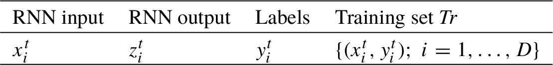
As is well known, in RNN prediction tasks, training sets are fed with temporal sequences composed with pairs of previous data of the form (input, labels) with the objective of predicting the future, referred to as future target value, y. Thus, ${X^{t}}$ is the time-varying variable which needs to be estimated, ${Z^{t}}$ is the set of RNN outputs and ${Y^{t}}$ the set of labels (i.e. past target values for training). In terms of the illustrative example: to predict the electrity price one month ahead (target value y, $t=+1$), the training sets are made up of temporal sequences $({x_{i}^{t}},{y_{i}^{t}})$ whose first component contains different factors that influence electricity prices (fuel prices, transmission and distribution costs, weather conditions, etc.) and whose second component is the electrity price, both ${x_{i}^{t}}$, ${y_{i}^{t}}$ in site i and prior to present time ($t=-9,\dots ,-2,-1,0$).
Let $\textit{In}$ be the (time-dependent) input RNN dataset formed by n vectors:
 ${Z^{t}}[\textit{In}]$ will stand for the set of outputs which is generated after the completed RNN process corresponding the the set of inputs $\textit{In}$.
\[ \textit{In}=\big\{{x_{i}^{t}}=\big({x_{i}^{1,t}},{x_{i}^{2,t}},\dots ,{x_{i}^{d,t}}\big),\hspace{2.5pt}i=1,\dots ,n\big\},\]
each of them contains d features: ${x_{i}^{j,t}}\in \mathbb{R}$, $i=1,\dots $, $n;j=1,\dots ,d$: The objective is to select from the n inputs in $\textit{In}$, $D\lt n$ vectors that will make up the training set: the selection criterion is to choose those which produce the best estimates in the RNN learning process. The choice will be conducted by only using prior probability –instead of posterior– and the VNM Theorem 2.1.
We will list the steps to be taken:
-
• Main lottery (in $\textit{In}$). The key idea is to adapt the scenario of the RNN learning process (inputs, outputs, labels, target value) to the situation described in the VNM-Theorem 2.1, and to rely on the TD-MRF methodology for computing the probabilities. To do so, we consider the process of selecting $D\lt n$ vectors as a lottery whose outcomes are the D vectors we have chosen for the training set (main lottery). Each of these D vectors has its own likelihood of being chosen.
-
• Consider the RNN process as composed by several uncertain processes, ${\textit{RNN}_{i}}$, one for each of the input vectors ${x_{i}^{t}}$ that make up the set $\textit{In}$, $i=1,\dots ,n$ (Fig. 1). After the RNN learning is completed, a set of n outputs ${Z^{t}}[\textit{In}]$ is generated. Note that, since RNN is deterministic (the same set of inputs will produce the same set of outputs), input ${x_{i}^{t}}$ has a uniquely associated output ${z_{i}^{t}}$.
-
• Secondary lottery (for each ${z_{i}^{t}}\in {Z^{t}}[\textit{In}]$). A second lottery arises for each output ${z_{i}^{t}}\in {Z^{t}}[\textit{In}]$ when the selection criterion is applied: how good the estimate ${z_{i}^{t}}$ is. If M denotes the threshold below which the loss function is considered acceptable, the secondary lottery is whether the loss function $\text{loss}({z_{i}^{t}})\lt M$ or not.To ensure that our selection rule is applied, we define a preference relation on $\textit{In}=\{{x_{i}^{t}},\hspace{0.1667em}i=1,\dots ,n\}$. Due to the unique existing direction from input ${x_{i}^{t}}$ to RNN output ${z_{i}^{t}}$, the preference relation can be considered defined on both the set of inputs $\textit{In}$ and the set of outputs ${Z^{t}}[\textit{In}]$. Moreover, for the evident bidirection between outcome ${z_{i}^{t}}$ and associated loss $\text{loss}({z_{i}^{t}})$, the distinction that many authors make between defining a preference relation on the set of outcomes X or defining it on the set of lotteries over X, named $\Delta X$, does not apply in our case:In later sections we will show that this preference relation verifies the properties necessary for the application of the VNM theorem.
Definition 3.1.
For ${z_{i}^{t}},{z_{j}^{t}}\in {Z^{t}}[\textit{In}]$, ${z_{i}^{t}}\prec {z_{j}^{t}}\Leftrightarrow \text{loss}({z_{j}^{t}})\lt \text{loss}({z_{i}^{t}})$, i.e. ${z_{j}^{t}}$ is preferred to ${z_{i}^{t}}$ if ${z_{j}^{t}}$ is a better estimate (smaller associated loss). Indifference comes with the equality: for ${z_{i}^{t}},{z_{j}^{t}}\in {Z^{t}}[\textit{In}]$ ${z_{i}^{t}}\sim {z_{j}^{t}}\Leftrightarrow \text{loss}({z_{i}^{t}})=\text{loss}({z_{j}^{t}})$. -
• We thus apply Theorem 2.1 for the main lottery: the expected utility of training set $\textit{Tr}$ is given by
-
• In order to compute the (prior) probabilities $po[{X^{t}}={x_{i}^{t}}]$, we shall equip the initial RNN data set with an undirected graph structure –with appropriate node and edge definitions– which will later be shown to be an MRF by application of central Theorem 4.4. This will be the development of Section 4.
4 The Abstract TD-MRF-Based Framework
Here, we first design an abstract graph-based framework that shall provide a model for a dynamic context of k sites and r filters for data discrimination (corresponding to r cliques) for which it will be shown that it is an TD-MRF under certain mild conditions. Such TD-MRF will be the core in the computation of prior probabilities $po[{X^{t}}={x_{i}^{t}}]$ of the VMN Theorem 2.1.
Let $\mathcal{S}$ be a set of k sites ${s_{i}}$, $\mathcal{S}=\{{s_{i}}|i=1,2,\dots ,k\}$ such that the variable may take different values depending on the site, ${X_{{s_{i}}}^{t}}$. For each site ${s_{i}}$, the variable ${X_{{s_{i}}}^{t}}$ can be disaggregated into a set of d characteristics which fully describes ${X_{{s_{i}}}^{t}}$ in the instant of time t: ${X_{{s_{i}}}^{t}}=({X_{{s_{i}}}^{1,t}},{X_{{s_{i}}}^{2,t}},\dots ,{X_{{s_{i}}}^{d,t}})$, with lower case ${x_{{s_{i}}}^{t}}=({x_{{s_{i}}}^{1,t}},{x_{{s_{i}}}^{2,t}},\dots ,{x_{{s_{i}}}^{d,t}})$ for the feature vector (i.e. a numerical vector corresponding to a realisation of the variable). We shall use indistinctly ${x_{{s_{i}}}^{t}}=({x_{{s_{i}}}^{1,t}},{x_{{s_{i}}}^{2,t}},\dots ,{x_{{s_{i}}}^{d,t}})$ or ${x_{i}^{t}}=({x_{i}^{1,t}},{x_{i}^{2,t}},\dots ,{x_{i}^{d,t}})$ either for upper and lower case. In a compact form, ${x_{i}^{j,t}}\in \mathbb{R},i=1,\dots ,k;j=1,\dots ,d$.
Remember that two random variables are equivalent if they have identical distribution. Then, we will define the edges by equivalently defining the neighbourhood $\mathcal{N}$ of a site: $\mathcal{N}({X_{{s_{i}}}^{t}})=\{{X_{{s_{j}}}^{t}}|\hspace{0.2778em}{X_{{s_{j}}}^{t}},{X_{{s_{i}}}^{t}}\hspace{0.2778em}\text{are equivalent}\}=\{{X_{{s_{j}}}^{t}}|P[{X_{{s_{j}}}^{t}}\leqslant x]=P[{X_{{s_{i}}}^{t}}\leqslant x]\hspace{0.1667em}\forall x\}$.
Definition 4.1 (TD-DGM).
A DGM $({\mathcal{S}^{t}},{\mathcal{N}^{t}})$ is defined as follows: sites are the elements of the set ${\mathcal{S}^{t}}$ through the identification ${s_{i}^{t}}\sim {X_{{s_{i}}}^{t}}$. Edges are defined through the neighbourhood $\mathcal{N}$ of a site ${s_{i}^{t}}$ as $\mathcal{N}({X_{{s_{i}}}^{t}})=\{{X_{{s_{j}}}^{t}}|P[{X_{{s_{j}}}^{t}}\leqslant x]=P[{X_{{s_{i}}}^{t}}\leqslant x]\hspace{0.1667em}\forall x\}$.
Remark 4.2 (Clean data).
It is worth highlighting that Definition 4.1 (that makes equal all random variables with identical probability distribution) avoids duplicates. This is particularly important when applied to the graphical model resulting from an RNN input dataset (clean data).
Recall that marginal distribution is also known as prior probability in contrast with the posterior distribution (the conditional one). From the former definition, sites in the same neighbourhood have the same prior probability. Moreover,
Proposition 4.3.
Sites which belong to the same neighbourhood have identical probability a posteriori.
Proof.
Let ${s_{i}}$, ${s_{j}}$ be two sites which belong to the same neighbourhood. From the Bayes’s theorem, one has 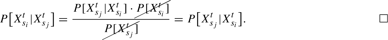
The following theorem proves then that the DGM defined in Definition 4.1 is a TD-MRF by equivalently showing that the Markov condition:
Proof.
We shall prove that the local dynamic Markov property is verified, i.e. the probability of ${X_{{s_{i}}}}$ conditioned to the remaining random variables, ${X_{{s_{j}}}},j\ne i$, is equal to the probability of ${X_{{s_{i}}}}$ conditioned to the random variables in the same neighbouring system ${X_{\mathcal{N}({s_{i}})}}$. The following development is considered in a specific time instant ${t_{0}}$. By assuming that the ${s_{i}}$-site estimation takes value ${x_{{s_{i}}}^{{t_{0}}}}$ while the rest does not (thus, their estimation is some $x\ne {x_{{s_{i}}}^{{t_{0}}}}$), we partition the set $\mathcal{S}$ as $\mathcal{S}-\{{s_{i}}\}=\mathcal{N}({s_{i}})-\{{s_{i}}\}\cup {\mathcal{N}_{ot}}({s_{i}})$, where ${\mathcal{N}_{ot}}({s_{i}})$ denotes those sites which are not in $\mathcal{N}({s_{i}})$. Thus,
\[\begin{aligned}{}P\big[{X_{{s_{i}}}^{{t_{0}}}}={x_{{s_{i}}}^{{t_{0}}}}\big|{X_{\mathcal{S}-\{{s_{i}}\}}^{{t_{0}}}}=x\ne {x_{{s_{i}}}^{{t_{0}}}}\big]& =\frac{P[({X_{{s_{i}}}^{{t_{0}}}}={x_{{s_{i}}}^{{t_{0}}}})\cap ({X_{\mathcal{S}-\{{s_{i}}\}}^{{t_{0}}}}=x\ne {x_{{s_{i}}}^{{t_{0}}}})]}{P[{X_{\mathcal{S}-\{{s_{i}}\}}^{{t_{0}}}}=x\ne {x_{{s_{i}}}^{{t_{0}}}}]}=\\ {} & =\frac{P[({X_{{s_{i}}}^{{t_{0}}}}={x_{{s_{i}}}^{{t_{0}}}})\cap ({X_{\mathcal{N}({x_{{s_{i}}}^{{t_{0}}}})}^{{t_{0}}}}=x\ne {x_{{s_{i}}}^{{t_{0}}}})]}{P[{X_{\mathcal{N}({x_{{s_{i}}}^{{t_{0}}}})}^{{t_{0}}}}=x\ne {x_{{s_{i}}}^{{t_{0}}}}]}=\\ {} & =P\big[{X_{{s_{i}}}^{{t_{0}}}}={x_{{s_{i}}}^{{t_{0}}}}\big|{X_{\mathcal{N}({x_{{s_{i}}}^{{t_{0}}}})}^{{t_{0}}}}=x\ne {x_{{s_{i}}}^{{t_{0}}}}\big].\end{aligned}\]
□Insofar as the distribution function is the tool used to make estimates, previous Theorem 4.4 provides a joint measure of how close the variable is to taking a particular value.
Corollary 4.5.
The corresponding Gibbs (joint) probability distribution at a time instant t provides that the likelihood of reaching a concrete value x is $P[{X^{t}}=x]=\frac{1}{Z}{\textstyle\prod _{\begin{array}{l}\textit{cliques}\hspace{2.5pt}{C_{j}}\\ {} \hspace{1em}j=1\end{array}}^{r}}{e^{-{\psi _{C}}({X^{t}}=x)}}$.
Each clique has its own common estimation function:
Proposition 4.7 (The cliques).
Each clique of the TD-MRF has its own estimation function given by the clique potentials ${e^{-{\psi _{{C_{j}}}}([.])}},j=1,\dots ,r$: ${P_{{C_{j}}}}[{X^{t}}=x]=\frac{1}{Z}{e^{-{\psi _{{C_{j}}}}({X^{t}}=x)}}$.
In discrimination/classification works, the commonly used probability is the conditional or posterior probability $P[{X^{t}}=x|y]=\frac{1}{Z}{\textstyle\prod _{\begin{array}{l}\text{cliques}\hspace{2.5pt}{C_{j}}\\ {} \hspace{1em}j=1\end{array}}^{r}}{e^{-{\psi _{C}}({X^{t}}=x|y)}}$ where x stands for RNN input, y represents the corresponding target value and ${\psi _{C}}({X^{t}}=x|y)$ means that the energy function ${\psi _{C}}$ only assigns to those inputs x that correspond to y.
4.1 Visual Flowchart of the TD-MRF Operational Process
Inputs for a TD-MFRs are specific values of the stochastic variable ${X^{t}}$ in a particular time instant t and a site ${s_{i}}$, ${x_{{s_{i}}}^{t}}$. Depending on the context, ${X^{t}}$ can be considered as disaggregated into a set of d features for each site ${s_{i}}$. Thus, each input is ${x_{i}^{t}}=({x_{i}^{1,t}},{x_{i}^{2,t}},\dots ,{x_{i}^{d,t}})$, ${x_{i}^{j,t}}\in \mathbb{R}$, $i=1,\dots ,k$, $j=1,\dots ,d$ such that each univariate component ${x_{i}^{j,t}}\in \mathbb{R}$ can be regarded as input of a single-variable for d processes. The TD-GDM operational process is as follows: by assuming there are r cliques, ${C_{1}},\dots ,{C_{r}}$, each input is processed in a clique ${\mathcal{C}_{j}},j=1,\dots ,r$, through the corresponding clique potential ${e^{-{\psi _{{C_{j}}}}([.])}},j=1,\dots ,r$, such that the output is the estimate made by the corresponding clique (according to Proposition 4.7). Each of these is thus aggregated in a final output by means of the expression given in Corollary 4.5. If, on the other hand, the variable is not considered disaggregated, multivariate energy functions will process the information in a single multivariate execution.
Figure 2 provides a visual representation of a TD-MRF operation in the univariate scenario, where the energy functions ψ are of Gaussian type, i.e. ${\psi _{{C_{j}}}}=\frac{{([.]-{\mu _{j}})^{2}}}{{\sigma _{j}^{2}}}$, $j=1,\dots ,r$. Note that for ${x_{i}^{t}}=({x_{i}^{1,t}},{x_{i}^{2,t}},\dots ,{x_{i}^{d,t}})$, the corresponding probability $po[{x_{i}^{t}}]$ is $po[{x_{i}^{t}}]=(po[{x_{i}^{1,t}}],po[{x_{i}^{2,t}}],\dots ,po[{x_{i}^{d,t}}])$.
Moreover, the operation of an MRF is equally applied in the calculation of following probabilities:
\[\begin{aligned}{}& {P_{{C_{j}}}}\big[{X^{t}}\leqslant {x^{t}}\big]=\sum \limits_{x\leqslant {x^{t}}}P\big[{X^{t}}=x\big],\\ {} & {P_{{C_{j}}}}\big[{x_{pr}}\lt {X^{t}}\leqslant {x_{im}}\big]=\sum \limits_{x\leqslant {x_{im}}}P\big[{X^{t}}=x\big]-\sum \limits_{i\leqslant {x_{pr}}}P\big[{X^{t}}=x\big],\\ {} & {P_{{C_{j}}}}\big[{X^{t}}\gt {x^{t}}\big]=1-{P_{{C_{j}}}}\big[{X^{t}}\leqslant {x^{t}}\big]=1-\sum \limits_{x\leqslant {x^{t}}}P\big[{X^{t}}=x\big].\end{aligned}\]
4.2 TD-MRF Structure for the RNN Input Set
Our goal here is to provide a graph-structure (which will become TD-MRF structure according to Theorem 4.4) for the set $\textit{In}$ of RNN inputs $\textit{In}=\{{x_{i}^{t}}=({x_{i}^{1,t}},{x_{i}^{2,t}},\dots ,{x_{i}^{d,t}}),i=1,\dots ,n\}$, each ${x_{i}^{j,t}}\in \mathbb{R}$, $i=1,\dots ,n$; $j=1,\dots ,d$.
To achieve this, the steps to follow are listed below:
-
1. The pre-processing phase. Before training/testing an RNN, data must suffer some preprocessing steps for removing duplicates, unnecessary information and simulating missing data. Depending on the context, data must also be normalised with feature scaling. We shall assume that RNN input datasets have completed this phase.
-
2. The input set graph structure. We endow the RNN data set with an undirected graph structure, according to Definition 4.1, where $k=D$:
-
• sites ${s_{i}^{t}}$ are the local version of the random variable ${X^{t}}$, i.e. the random variable ${X_{i}^{t}}$ for which the set of inputs ${x_{i}^{t}}$ are a realisation of it: ${s_{i}^{t}}={X_{{s_{i}}}^{t}}$.
-
• The neighbourhood of a site is defined as\[\begin{aligned}{}\mathcal{N}\big({X_{{s_{i}}}^{t}}\big)& =\big\{{X_{{s_{j}}}^{t}}\big|{X_{{s_{j}}}^{t}},{X_{{s_{i}}}^{t}}\hspace{0.2778em}\text{are equivalent}\big\}\\ {} & =\big\{{X_{{s_{j}}}^{t}}\big|P\big[{X_{{s_{j}}}^{t}}\leqslant x\big]=P\big[{X_{{s_{i}}}^{t}}\leqslant x\big]\hspace{0.1667em}\forall x\big\}.\end{aligned}\]in the sense of Definition 4.1. According to Remark 4.2, this definition is intended for discarding duplicates in the datasets.
-
-
3. The corresponding Gibbs distribution. According to Theorem 4.4, the graphical model formed by the RNN input data viewed as a time varying random variable ${X^{t}}$ is TD-MRF, with a Gibbs distribution $P[{X^{t}}]=\frac{1}{Z}{\textstyle\prod _{\text{cliques}\hspace{2.5pt}C}}\exp [-{\psi _{C}}({X^{t}})]$.
-
4. Likelihood of occurrence of an output. Recall that from Definition 4.1, neighbours are equal to cliques and both consist of those random variables which have equal prior distributions (and identical posterior distribution in consequence). Hence, a probability $po[{X^{t}}={x_{i}^{t}}]$ is biunivocally determined for each input ${x_{i}^{t}}$. We also refer to Fig. 2 to reproduce the operation of an TD-MRF in a single multivariate execution.
5 Application of the VNM Utility Theorem
In this section, we will further develop equation (3),
\[ u[\textit{Tr}]=u\big[\big\{{x_{1}^{t}},\dots ,{x_{D}^{t}}\big\}\big]={\sum \limits_{i=1}^{D}}po\big[{X^{t}}={x_{i}^{t}}\big]\cdot u\big({x_{i}^{t}}\big),\]
by giving the explicit calculation of $u({x_{i}^{t}})$, $\forall i$, t. To do so, we will again apply the VMN theorem to the secondary lottery.Recall that in the preceding sections we have considered a second lottery which arises naturally when we test how good the ouput ${z_{i}^{t}}\in {Z^{t}}[\textit{In}]$ is as estimate. If M is the threshold below which the loss function is considered acceptable, the secondary lottery is whether the loss function $\text{loss}({z_{i}^{t}})\lt M$ or not. With the intuitive notation of the paper (Machina, 1982), our secondary lottery is a probability distribution function over the interval $[0,M]$ (the set of all lotteries over $[0,M]$ is denoted in Machina (1982) by $D[0,M]$) and the preference functional $V(\cdot )$ on $D[0,M]$ in our case is $\text{loss}(\cdot )$. Note that Definition 3.1 of preference over the set ${Z^{t}}[\textit{In}]$ can be additionally considered over $\textit{In}$ for the deterministic assignment ${x_{i}^{t}}\to {z_{i}^{t}}$: for ${x_{i}^{t}},{x_{j}^{t}}\in \textit{In}$
\[ {x_{i}^{t}}\prec {x_{j}^{t}}\Leftrightarrow {z_{i}^{t}}\prec {z_{j}^{t}}\Leftrightarrow \text{loss}\big({z_{j}^{t}}\big)\lt \text{loss}\big({z_{i}^{t}}\big),\]
where the loss function is considered in a squared-form, $\text{loss}({z_{i}^{t}})={({z_{i}^{t}}-{y_{i}})^{2}}$ which in the context or real positive numbers is equivalent to $\text{loss}({z_{i}^{t}})=|{z_{i}^{t}}-{y_{i}}|$. The objective here is to prove that this binary relation satisfies the necessary conditions that enable the application of the Von Neumann-Morgenstern (VNM) theorem.First of all, it has to be shown that it is a preference relation:
Proof.
The standard axiom for a preference relation is rationality which includes both completeness and transitivity.
□
-
• Completeness: for all ${z_{i}^{t}},{z_{j}^{t}}\in {Z^{t}}[\textit{In}]$, either ${z_{i}^{t}}\preceq {z_{j}^{t}}$ or ${z_{i}^{t}}\succeq {z_{j}^{t}}$. This property comes from the fact that $\mathbb{R}$ has a total order when applying to $|{z_{i}^{t}}-{y_{i}}|,|{z_{j}^{t}}-{y_{i}}|\in \mathbb{R}$.
-
• Transitivity: for all ${z_{i}^{t}},{z_{j}^{t}},{z_{l}^{t}}\in {Z^{t}}[\textit{In}]$, if ${z_{i}^{t}}\preceq {z_{j}^{t}}$ and ${z_{j}^{t}}\preceq {z_{l}^{t}}$, thus ${z_{i}^{t}}\preceq {z_{l}^{t}}$. This property holds by the transitivity in the order of $\mathbb{R}$: $|{z_{i}^{t}}-{y_{i}}|\leqslant |{z_{j}^{t}}-{y_{i}}|\leqslant |{z_{l}^{t}}-{y_{i}}|$ $\Rightarrow |{z_{i}^{t}}-{y_{i}}|\leqslant |{z_{l}^{t}}-{y_{i}}|$.
Moreover, former preference relation satisfies the following conditions:
Proof.
Continuity: let us prove that if each element ${z_{n}^{t}}$ of a sequence of outcomes is ${z_{n}^{t}}\succeq z$, thus it must be ${\lim \nolimits_{n\to \infty }}{z_{n}^{t}}\succeq z$. First, we have that
\[\begin{aligned}{}{\big({z_{n}^{t}}-{y_{n}}\big)^{2}}& ={\big({z_{n}^{t}}\big)^{2}}-2{z_{n}^{t}}\cdot {y_{n}}+{y_{n}^{2}}\Rightarrow \\ {} \underset{n\to \infty }{\lim }{\big({z_{n}^{t}}-{y_{n}}\big)^{2}}& =\underset{n\to \infty }{\lim }{\big({z_{n}^{t}}\big)^{2}}-\underset{n\to \infty }{\lim }\big(2{z_{n}^{t}}\cdot {y_{n}}\big)+\underset{n\to \infty }{\lim }{y_{n}^{2}}=\\ {} & =\underset{n\to \infty }{\lim }{\big({z_{n}^{t}}\big)^{2}}-2\underset{n\to \infty }{\lim }{z_{n}^{t}}\cdot \underset{n\to \infty }{\lim }{y_{n}}+\underset{n\to \infty }{\lim }{y_{n}^{2}}=\\ {} & ={\big(\hspace{0.1667em}\underset{n\to \infty }{\lim }{z_{n}^{t}}-\underset{n\to \infty }{\lim }{y_{n}}\big)^{2}}.\end{aligned}\]
Let us suppose that ${z_{n}^{t}}$ is a sequence of outcomes such that ${z_{n}^{t}}\succeq z$, that is, output z is preferred to outputs ${z_{n}^{t}}$. That means that ${(z-y)^{2}}\lt {({z_{n}^{t}}-{y_{n}})^{2}}$ where y, ${y_{n}}$ are the corresponding target values for the inputs that correspond to z and ${z_{n}^{t}}$, respectively.
By assuming that both limits exist, the inequality ${(z-y)^{2}}\lt {({z_{n}}-{y_{n}})^{2}}$ is preserved in “less than or equal” form: ${\lim \nolimits_{n\to \infty }}{(z-y)^{2}}={(z-y)^{2}}\leqslant {\lim \nolimits_{n\to \infty }}{({z_{n}^{t}}-y)^{2}}$. Hence,
Fréchet differentiable. Recall that the Fréchet derivative in finite-dimensional spaces is the usual derivative. Thus, the loss function $\text{loss}({z_{i}^{t}})={({z_{i}^{t}}-y)^{2}}$ verifies this hypothesis. □
Therefore, the preference relation stated in Definition 3.1 verifies the conditions required for the application of the VNM Theorem 2.1. Thus, there exists an utility function $u:\textit{In}\to [0,1]$ which quantifies the preferences: ${x_{1}^{t}}\succeq {x_{2}^{t}}$ iff $u({x_{1}^{t}})\geqslant u({x_{2}^{t}})$. Moreover, the Von Neumann-Morgenstern Expected Utility theorem also provides guidance for computing the utility of the set of inputs through the explicit formula given in equation (3):
6 Main Results
The objective of this section is to highlight (after proving) the main results of our proposal. First of all, we define the level of efficiency of an input set $\textit{In}$, $\text{Eff}[\textit{In}]$. Thus, next Theorem 6.2 proves the existence of a formula for determining the efficiency of a training set while Theorem 6.3 gives an explicit expression for computing $\text{Eff}[\textit{In}]$.
Definition 6.1.
We define the level of efficiency of an input set $\textit{In}$, $\text{Eff}[\textit{In}]$ as the expected utility of training set $\textit{Tr}$: $\text{Eff}[\textit{In}]:=u[\{{x_{1}^{t}},\dots ,{x_{D}^{t}}\}]={\textstyle\sum _{i=1}^{D}}po[{X^{t}}={x_{i}^{t}}]\cdot u({x_{i}^{t}})$.
Theorem 6.2 (Existence).
For any input set $\textit{In}$, there exists an utility function $u:\textit{In}\to [0,1]$ which allows to quantify its level of efficiency $\textit{Eff}[\textit{In}]$ such that this can be computed as
Proof.
Following Proposition 5.2, the preference relation stated in Definition 3.1 verifies the necessary conditions for applying the VNM Theorem 2.1. According to this, there exists an utility function $u:\textit{In}\to [0,1]$, which quantifies the preferences over input vectors: ${x_{1}^{t}}\succeq {x_{2}^{t}}$ iff $u({x_{1}^{t}})\geqslant u({x_{2}^{t}})$. □
Theorem 6.3 (How to compute the level of efficiency of $\textit{In}$).
We assume that all inputs are equally distributed. Thus, for any RNN input set $\textit{In}$, its level of efficiency can be explicitely computed as
Proof.
We start from expression $\text{Eff}[\textit{In}]={\textstyle\sum _{i=1}^{D}}po[{X^{t}}={x_{i}^{t}}]\cdot u({x_{i}^{t}})$ derived from Theorem 6.2. On one hand, the explicit computation of probabilities ${\{po[{X^{t}}={x_{i}^{t}}]\}_{i=1}^{D}}$ is given by the TD-MRF operational process defined in Section 4 (see Fig. 2, which visually describes this). On the other hand, in order to compute the utilities ${\{u({x_{i}^{t}})]\}_{i=1}^{D}}$, we shall apply again the VNM Theorem 2.1 for the secondary lottery. Recall that the secondary lottery for each ${z_{i}^{t}}$ is whether the loss function $|{z_{i}^{t}}-y|\lt M$ or not, for a given threshold M below which the loss function is considered acceptable. Recall also that the probability of occurrence of an RNN output $po[{z_{i}^{t}}]$ is $po[{z_{i}^{t}}]=po[{X^{t}}={x_{i}^{t}}]$. To overcome a continuous space of outcomes ${\{|{z_{i}^{t}}-y|\in \mathbb{R}\}_{i=1}^{D}}$ for the lottery associated to each ${z_{i}^{t}}$, we represent it in a binary form:
\[ \left\{\begin{array}{l@{\hskip4.0pt}l}\text{outcome}\hspace{2.5pt}1\hspace{1em}& \text{if}\hspace{2.5pt}|{z_{i}^{t}}-y|\lt M,\\ {} \text{outcome}\hspace{2.5pt}0\hspace{1em}& \text{if}\hspace{2.5pt}|{z_{i}^{t}}-y|\geqslant M.\end{array}\right.\]
Since the utility function u represents a set of outcomes in the sense of VNM-theorem 2.1 (${x_{1}}\succeq {x_{2}}$ iff $u({x_{1}})\geqslant u({x_{2}})$), we can conclude that
\[ \left\{\begin{array}{l@{\hskip4.0pt}l}\text{outcome}\hspace{2.5pt}1\hspace{1em}& \text{if}\hspace{2.5pt}|{z_{i}^{t}}-y|\lt M\Rightarrow u(1)=1,\\ {} \text{outcome}\hspace{2.5pt}0\hspace{1em}& \text{if}\hspace{2.5pt}|{z_{i}^{t}}-y|\geqslant M\Rightarrow u(0)=0.\end{array}\right.\]
Then, by application of VNM-Theorem 2.1 on each secondary lottery, one has that
\[\begin{aligned}{}& u\big({x_{i}^{t}}\big)=u\big({z_{i}^{t}}\big)\\ {} & \hspace{1em}={\sum \limits_{i=1}^{2}}p[{\text{outcome}_{i}}]\cdot u({\text{outcome}_{i}})=p[\text{outcome}\hspace{2.5pt}1]\cdot 1=p[\text{outcome}\hspace{2.5pt}1],\\ {} & \hspace{2em}\forall i=1,\dots ,D.\end{aligned}\]
The formula comes then by substituting:
\[\begin{aligned}{}\text{Eff}[\textit{In}]& ={\sum \limits_{i=1}^{D}}po\big[{X^{t}}={x_{i}^{t}}\big]\cdot u\big({x_{i}^{t}}\big)=\\ {} & ={\sum \limits_{i=1}^{D}}po\big[{X^{t}}={x_{i}^{t}}\big]\cdot p[\text{outcome}\hspace{2.5pt}1]=\\ {} & =p[\text{outcome}\hspace{2.5pt}1]\cdot {\sum \limits_{i=1}^{D}}po\big[{X^{t}}={x_{i}^{t}}\big]=\\ {} & =p\cdot {\sum \limits_{i=1}^{D}}po\big[{X^{t}}={x_{i}^{t}}\big].\end{aligned}\]
□7 A Case Application
This section is aimed at developing an example of the method application. In order to make a choice between two real data sets, their level of efficiency will be computed. As stated in Definition 6.1, the level of efficiency of an input set $\text{Eff}[\textit{In}]$ measures the learning capacity of its inputs on the basis of the preference relation of Definition 3.1 that prioritises those inputs whose outputs have a lower associated loss (better estimates). To compute $\text{Eff}[{I_{n}}]$ we shall apply the formula proved in Theorem 6.3 which follows from Theorem 6.2, in which the existence of an utility function u which quantifies the preference relation was proved. This is
\[ \text{Eff}[\textit{In}]={\sum \limits_{i=1}^{D}}po\big[{X^{t}}={x_{i}^{t}}\big]\cdot u\big({x_{i}^{t}}\big)=p\cdot {\sum \limits_{i=1}^{D}}po\big[{X^{t}}={x_{i}^{t}}\big],\]
where p is the probability that $|{z_{i}^{t}}-y|\lt M,\forall {z_{i}^{t}}$ for a given threshold M below which the loss function is considered acceptable.The data sets we shall use here contain prices (€/1 kg) over time for the most common olive oil varieties. These data are available on the websites of the Government of Spain:
where prices are published on a weekly basis. Specifically, we will consider data sets corresponding to weeks 28/2023 and 39/2022 (the reasons for this choice will be explained later). We shall thus apply the above formula taking into account the following considerations. On one hand, note that the choice of the threshold M will depend on the context. In the olive oil market scenario, assuming a deviation from the olive oil price of 10% is acceptable. Hence, $M=0.5$. On the other hand, the value of the parameter p will depend on several market features which vary over time depending on physical (rainfall, pollen levels$\dots \hspace{0.1667em}$) and socio-economic (Government regulations) circumstances. When real prices are subject to unusual fluctuations (due to changes in the aforementioned circumstances), such prices used in training tasks will deviate more from the real ones. In consequence, the probability p, such that $|{z_{i}^{t}}-y|\lt M,\forall {z_{i}^{t}}$, will decrease. Either way, it should be noticed that p is known as soon as the value of M is fixed, but it is not the same for all input sets.
From the above formula, since M is known (and therefore so is p), we must focus on computing $po[{X^{t}}={x_{i}^{t}}]$ for each input ${x_{i}^{t}}$. To that end, we will follow Fig. 2 of the TD-MRF operational process given in Section 4.1. Since each input ${x_{i}^{t}}$ may be disaggregated into d features ${x_{i}^{k,t}}$ ($k=1,\dots ,d$), ${x_{i}^{t}}=({x_{i}^{1,t}},{x_{i}^{2,t}},\dots ,{x_{i}^{d,t}})$, the same is true for the corresponding probability $po[{X^{t}}={x_{i}^{t}}]=po[{x_{i}^{t}}]$, which is $po[{x_{i}^{t}}]=(po[{x_{i}^{1,t}}],po[{x_{i}^{2,t}}],\dots ,po[{x_{i}^{d,t}}])$.
We assume that the energy functions ψ corresponding to the r cliques are of Gaussian type, i.e. ${\psi _{{C_{j}}}}=\frac{{([.]-{\mu _{j}})^{2}}}{{\sigma _{j}^{2}}}$, $j=1,\dots ,r$, since Gaussian distributions are suitable in the olive oil scenario. Actually, given that Gaussian distributions portray those data sets whose majority of elements revolves around the centre, energy functions of Gaussian type are particularly suited for goods whose price takes values in an interval of small length and do not suffer very sharp price variations.
In order to achieve our goal, each input ${x_{i}^{t}}$ must be first processed in each clique ${\mathcal{C}_{j}},j=1,\dots ,r$, through the corresponding clique potential, whose result is
\[ {P_{{C_{j}}}}\big[{X^{t}}={x_{i}^{t}}\big]=\frac{1}{Z}{e^{-\frac{{({x_{i}^{t}}-{\mu _{j}})^{2}}}{{\sigma _{j}^{2}}}}}\Rightarrow {P_{{C_{j}}}}\big[{X^{t}}={x_{i}^{t}}\big]={e^{-\frac{{({x_{i}^{t}}-{\mu _{j}})^{2}}}{{\sigma _{j}^{2}}}}},\hspace{1em}\text{when}\hspace{2.5pt}Z=1.\]
Once the processing in the cliques has been completed, the required probability is obtained as
\[\begin{aligned}{}& po\big[{x_{i}^{t}}\big]=P\big[{X^{t}}={x_{i}^{t}}\big]=\frac{1}{Z}{\prod \limits_{j}^{r}}{P_{{C_{j}}}}\big[{X^{t}}={x_{i}^{t}}\big]\Rightarrow P\big[{X^{t}}={x_{i}^{t}}\big]={\prod \limits_{j}^{r}}{e^{-\frac{{({x_{i}^{t}}-{\mu _{j}})^{2}}}{{\sigma _{j}^{2}}}}},\\ {} & \hspace{1em}\text{when}\hspace{2.5pt}Z=1.\end{aligned}\]
The computation of “the partition function” Z entails certain difficulties in practice. For this reason, we shall adopt the view commonly taken in the literature that $Z=1$.From the TD-MRF structure proved in Theorem 4.4, cliques gather those random variables with identical prior and posterior distribution (see Remark 4.6). This theoretical description fits with the specialist major retailers in the olive oil context. In this practical case, the level of efficiency shall be computed through ${P_{{C_{j}}}}[{X^{t}}={x_{i}^{t}}]$ of cliques ${C_{j}},\hspace{0.1667em}j=1,\dots ,7$ supported by the information given in Table 8 below (source: https://www.olimerca.com/precios/tipoInforme/3).
As discussed before, there are multiple factors (physical and socio-economic) that influence the price. Such factors are the features ${x_{i}^{k,t}}$ ($k=1,\dots ,d$) of each input ${x_{i}^{t}}=({x_{i}^{1,t}},{x_{i}^{2,t}},\dots ,{x_{i}^{d,t}})$. For simplicity, we focus on just one of them in order to choose the two input sets ${\textit{In}_{1}},{\textit{In}_{2}}$: the hydrographic index, which shows the average rainfall over a certain period of time. In this line, ${\textit{In}_{1}}$ is an input set of prices (€/1 kg) under severe drought conditions (and therefore, with unusual fluctuations in price as product shortages raise the prices3) while ${\textit{In}_{2}}$ is an input set of prices which correspond to a usual period of rainfall:
\[\begin{aligned}{}{\textit{In}_{1}}& =\{3.16,5.92,6.26,6.52,7.10\},\hspace{2.5pt}p=0.23,\hspace{1em}\text{week}\hspace{2.5pt}28/2023,\\ {} {\textit{In}_{2}}& =\{2.71,3.78,3.80,3.86,3.96\},\hspace{2.5pt}p=0.57,\hspace{1em}\text{week}\hspace{2.5pt}39/2022.\end{aligned}\]
With this choice of ${\textit{In}_{1}}$ and ${\textit{In}_{2}}$, it is to be expected that the inputs in ${\textit{In}_{1}}$ will produce worse estimators (higher associated loss) since such inputs reflect prices with unusual fluctuations (therefore with higher deviation from the mean). Hence, it is is to be expected that $\text{Eff}[{\textit{In}_{2}}]\gt \text{Eff}[{\textit{In}_{1}}]$.The computation of level of efficiency ${\textit{In}_{1}}$ is supported by the information provided in Tables 1–7.
Table 8
Mean and variance of cliques ${C_{1}}-{C_{7}}$.
| Mean, Variance | ${C_{1}}$ Ahorramas | ${C_{2}}$ Alcampo | ${C_{3}}$ Carrefour | ${C_{4}}$ Dia | ${C_{5}}$ Hipercor | ${C_{6}}$ Lidl | ${C_{7}}$ Mercadona |
| ${\mu _{i}}$ | 3.988 | 3.884 | 3.851 | 3.858 | 4.343 | 3.878 | 3.916 |
| ${\sigma _{i}^{2}}$ | 0.172 | 0.156 | 0.143 | 0.108 | 0.472 | 0.134 | 0.117 |
From the information provided by the above tables, finally the required probability is computed (see Table 9).
$\text{Eff}[{\textit{In}_{1}}]=p\cdot (po[{X^{t}}=3.16]+po[{X^{t}}=5.92]+po[{X^{t}}=6.26]+po[{X^{t}}=6.52]+po[{X^{t}}=7.10])=0.23\cdot (2.09102\text{E}-12+2.55039\text{E}-74+3.7242\text{E}-101+1.7143\text{E}-124+2.4066\text{E}-185)=0.23\cdot 2.09102\text{E}-12=$
Similarly, the computation of ${\textit{In}_{2}}$ is supported by the information provided in Tables 10–16.
Finally, the required probability is computed (see Table 17).
$\text{Eff}[{\textit{In}_{2}}]=p\cdot (po[{X^{t}}=2.71]+po[{X^{t}}=3.78]+po[{X^{t}}=3.80]+po[{X^{t}}=3.86]+po[{X^{t}}=3.96])=0.57(3.24825\text{E}-30+0.268808808+0.337851876+0.53631732+0.549630567+1.692608571)=$ .
.
Hence, as expected (since the inputs of ${\textit{In}_{1}}$ reflect prices with unusual fluctuations and therefore with higher deviation from the mean) $\text{Eff}[{\textit{In}_{2}}]\gt \text{Eff}[{\textit{In}_{1}}]$.
8 Conclusions
This paper deals with the selection of optimal training sets (those that have a higher capacity as estimators) in Recurrent Neural Networks under prediction tasks (or pattern recognition with time series as inputs), although this may also apply to other data-driven models regulated by dynamic systems. Our objective is to fill the existing gap of clear guidelines to follow for selecting optimal training sets in a general context.
We design here a novel methodology to select optimal training data sets that can be used in any context. The key idea, which underpins the design of the mathematical structure that supports the selection, is a binary relation that gives preference to inputs with higher estimator abilities. A second novelty of our approach is to use dynamic tools that have not been used previously for this purposes: dynamic Markov Networks, which are widely regarded as generative models, successfully compute the prior probabilities involved in the formula for calculating the degree of efficiency of the training set (Theorem 6.3), derived from application of the Von Neumann-Morgenstern Theorem 2.1. It is precisely the VMN theorem the instrument that confers discriminative capacity to the MNs: in this work we show that the preference relation that we define between inputs of a training set (inputs with higher learning capacities are preferred in the sense that the error function takes lower values) fulfils the necessary hypotheses to derive the existence of a simple formula for the calculation of the utility (efficiency) of a training set.
The simplicity of this calculation allows it to be carried out in parallel with the learning process without adding computational cost. Thus the optimal sets are selected as the learning process evolves, therefore the data noise gradually disappears which decreases the likelihood of overfitting occurring.
Declarations of interest: none.