1 Introduction
Industrial processes are immanently nonlinear, inertial, with time delays and variable parameters (Stephanopoulos,
1984), and hence difficult to be modelled and controlled. The fuzzy logic controllers (FLCs) are successful in ensuring of robust and high performance control for various processes (Driankov and Hellendoorn,
2001; Kosko,
1992) without explicit mathematical plant model. However, the bad impact of a high plant time delay on the system performance and stability requires a special compensation.
There are two ways to compensate the high plant time delay – by Smith predictor controllers and by plant predictors. The classical Smith predictor is developed for linear time-invariant plants (Stephanopoulos,
1984). In Yordanova (
2011), Yordanova (
2012) this technique is extended for nonlinear plants on the basis of a Takagi-Sugeno-Kang (TSK) fuzzy dynamic plant model and a TSK fuzzy logic controller on the principle of parallel distributed compensation (PDC), suggested first in Tanaka and Wang (
2001). The TSK model ensures soft switching among several linear models, valid for different operation zones. The fuzzy PDC is built of local linear controllers in the rule conclusions, Smith predictors in this case. Each local Smith predictor is designed for each local linear plant with time delay using the well mastered linear control technique. The TSK-PDC concept enables the study of the global PDC-Smith predictor system stability by application of the Lyapunov indirect method and the linear matrix inequalities (LMIs) numerical technique (Yordanova,
2011). Various plant predictors are suggested in Flores
et al. (
2005), Mahfouf
et al. (
2001), Yahsunobu and Hasegawa (
1986), Yordanova (
2011), Yordanova
et al. (
2006). They are based on fuzzy, neural and neuro–fuzzy (NF) integrated techniques (Jang,
1993; Jang
et al.,
1997; Kosko,
1992) for easy mapping of nonlinear relationships, robustness to imprecision and uncertainties, learning from experience (experimental data) and adaptation. The training of the predictor is off–line and facilitated greatly by the large number of developed software (Fuzzy Logic Toolbox,
1992; IEC,
1999; Jang,
1993; SIMATIC S7,
2002). In Babuška
et al. (
1999), Castellano (
2000), Mendonça
et al. (
2004) a Sugeno or a NF predictor is used in the generalized model predictive control (GMPC) scheme (Camacho and Bordons,
2004; Clarke
et al.,
1987; Rawlings and Mayne,
2009). Predictive FLCs are demonstrated for different applications. In Mahfouf
et al. (
2001) a predictive FLC is developed for level control on the basis of a TSK plant model. In Mazinan and Sadati (
2010) a multi-model linear predictive control on local FLCs and one–step fuzzy predictors in series is suggested for tubular heat exchanger. A predictive FLC is applied for air-conditioning with an internal plant model in Sousa
et al. (
1997) and with a Sugeno neuro-fuzzy plant predictor (NFPP) in Thompson and Dexter (
2005). In Yahsunobu and Hasegawa (
1986) a predictive FLC is designed for crane control and in Marsili-Libelli and Colzi (
1998) – for diffusion processes, where the rate of error is substituted by a NF error prediction. A NFPP is trained from plant simulation data and a FLC is designed based on an inverse cause–result relationship for the metal position control in sinter strand process in Hu and Rose (
1997). An optimization of fuzzy model predictive controller using genetic algorithms (GAs) is presented in Sarimveis and Bafas (
2003).
All existing approaches suffer the following common problems. The design methodology is complicated, application–bound and incomplete. It requires much initial data about the plant. No closed loop system stability analysis, validation of the models, theoretical justification of the parameters tuning and estimation of the proper prediction horizon are considered. The algorithms are computationally heavy, thus restricting their large scale real time industrial implementation via PLCs or embedded technique. The estimation of the improvements resulting from the effective compensation of the plant inertia and the high relative time delay is based mainly on simulations. The impact of important factors, observed in real time control and in industrial environment, such as noise, disturbances, sample time, restrictions on real signals (Kuo,
1995; Randall,
2002), plant nonlinearities, uncertainties, etc., related with the process, the measuring devices and the final control elements (Stephanopoulos,
1984), etc. are not accounted for.
Partial solution of the above problems is suggested in Yordanova
et al. (
2006), Yordanova and Mladenov (
2008) where the algorithm and the design are simplified by the introduction of a Sugeno NFPP in the system feedback. The NFPP is trained from simulation based on an approximate plant nonlinear model or experimental data using the MATLAB™ application Adaptive Neuro–Fuzzy Inference System (ANFIS) (Jang,
1993). The designed NF predictive controller (NFPC) can be easily programmed in an industrial programmable logic controller (PLC) (SIMATIC S7,
2002). A NFPC with a Sugeno NF main controller is developed for the processes of anaerobic digestion of organic waste in wastewater treatment in Yordanova
et al. (
2006), and the closed loop system stability and performance improvement studied by simulation from the linguistic phase trajectories and the step responses to reference, disturbance and model parameter changes. A NFPC with a linear PI main controller is developed and implemented for the real time liquid temperature control in a laboratory tank in Yordanova and Mladenov (
2008). The Sugeno NFPP is trained and validated using experimental data from the real time PI temperature control. The PI controller is empirically tuned using average for the range of operation plant model parameters estimated by plant identification or experts. The performance improvement – a reduced overshoot of the PI-NFPC system in regard to the PI control system, is assessed from one step response in real time control.
The aim of the present investigation is to develop a general, application–independent and experimentation–based methodology for the design of simple NF predictive controllers for compensation of the inertia and the high relative time delay of a nonlinear plant. The controller is built of a main FLC and a feedback Sugeno NFPP and is PLC feasible for real time industrial implementation. Its model-free design is based on selection of a proper prediction horizon, system stability analysis, GAs optimization, validation and assessment of the NFPC system performance improvement using data from real time control.
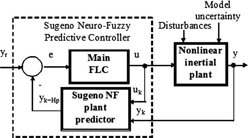
Fig. 1
Closed loop system with main FLC and feedback Sugeno NF plant predictor.
The closed loop system to be designed is shown in Fig.
1. It consists of a Sugeno NF predictive controller of type FLC-NFPP for the control of a nonlinear inertial plant with time delay. The notations are:
${y_{r}}$ is the reference;
$y(t)$ – the plant output controlled variable;
$u(t)$ – the control action;
${y_{k}}$ and
${u_{k}}$ are their values at discrete time
${t_{k}}$;
${y_{k+{H_{p}}}}$ – the predicted plant output for a prediction horizon
${H_{p}}$;
$e(t)={y_{r}}-{y_{k+{H_{p}}}}$ – the system error. The existence of a plant time delay
τ means that the current measured control
${u_{k}}$ will be felt at the plant output after
d sample periods
$\Delta t-{y_{k+d}}$, where
$\tau \approx d\Delta t$, or the current measured output
${y_{k}}$ is a result of a previous control
${u_{k-d}}$. A nonlinear plant determines a nonlinear plant predictor. A general approach for modelling of a nonlinear element – a plant predictor or a plant, is training of a neural network or a more economic in structure Sugeno NF system from pre-processed experimental plant input-output data. Sugeno models can model any nonlinearity with a small number of rules and membership functions (MFs). The plant time delay
τ can be compensated by selection of a proper prediction horizon
${H_{p}}$ even when
τ and all other nonlinear plant model parameters change with the operation point, defined by the plant inputs – control and disturbances, and the plant output. The role of the NFPP is to predict the expected after the time delay plant output.
The main tasks to be solved in the present research are:
-
– a TSK plant modelling and validation based on data from the real time plant control by an empirically designed model–free FLC;
-
– a Sugeno NFPP training and validation using experimental data from the FLC real time plant control and selection of a proper prediction horizon via investigations based on system simulations;
-
– stability analysis of the FLC-NFPP closed loop system using Lyapunov-LMIs approach and the TSK-PDC system representation based on a PDC GAs approximation of the FLC-NFPP and PDC validation using data from the FLC-NFPP real time control; the simpler PDC enables a PLC implementation;
-
– an assessment of the NFPC system performance improvement in regard to the performance of the FLC system from their real time operation for various reference changes. A comparison with alternative existing approaches is incorrect because of the more complex algorithms used which may not fit the real time control limitations, and the more sophisticated design based on a plant model and specific software.
The solutions of the above problems outline a novel general systematic approach for the design of computationally simple and experimentally proven FLC-NFPP. The design is illustrated for the air temperature in a laboratory dryer.
The input data is minimal initial empirical and/or expert information about the nonlinear inertial plant and its linear operation ranges needed for the design of a model-free Mamdani FLC and a TSK plant model.
The GAs are selected as a proper gradient-free optimization technique for random parallel search of global extremum of a nonlinear multimodal cost function of many parameters, defined often on experimental data and combining several criteria and constraints. They are frequently employed for tuning of FLCs, PDCs and other controllers from experimental data (Sarimveis and Bafas,
2003; Yordanova and Sivchev,
2014). A TSK model and a PDC are accepted to approximate the plant and the designed compound NFPC of a main FLC and a NFPP respectively. The grounds are that a TSK model can describe with desired accuracy any smooth sector–bounded, continuous nonlinear function and for each TSK plant model there always can be designed a corresponding PDC controller (Tanaka and Wang,
2001).
The investigations are carried out by the help of MATLAB™ and its toolboxes Simulink, Fuzzy logic, ANFIS (Fuzzy Logic Toolbox,
1992; Jang,
1993), Genetic algorithms (MATLAB – Genetic Algorithm,
2004), Real time (Real– Time Workshop,
2002) and Robust control with LMIs (Balas
et al.,
2005).
The rest of the paper is organized as follows. Section
2 is devoted to the derivation and the validation of a TSK plant model based on GAs parameter optimization and data from the real time control of a plant by a designed model-free main FLC. In Section
3 a NFPP is trained and validated, and a proper prediction horizon selected via simulation investigations. The NFPC system stability analysis, based on a PDC approximation of the NFPC, is presented in Section
4. In Section
5 the performance of the FLC-NFPP real time temperature control is assessed in regard to the performance of the FLC real time control. The conclusion and the future research are outlined in Section
6.
2 TSK Plant Modelling and Validation
First, a model-free FLC is designed and implemented for the real time control of the existing plant (pilot or industrial) to collect data for the TSK plant modelling.
The plant used to illustrate the developed approach is a small-scale laboratory tunnel dryer (Yordanova,
2011). The controlled variable
y is the air temperature in the tunnel, measured by the help of an industrial transducer platinum 100 for temperatures
${[0,200]^{\circ }}$C with a three-wired connection to a transmitter with voltage output in the range
$[0,10]$ V. The industrial final control elements are an electrical heater, a fan and a solid state relay (SSR) to connect them to the nets voltage supply during the pulses of a Pulse-Width-Modulator (PWM). The cooling is by natural convection. The plant is smoothly nonlinear and inertial. A data acquisition board (DAQ) with an Analog-to-Digital Converter (ADC) and a Digital Output (DO) constitutes the interface between the dryer and a computer. A MATLAB™-Simulink model performs the real time control at each discrete time moment reading via the ADC of the DAQ the voltage of the temperature transmitter, converting it to measured temperature, computing the system error, evaluating the control action
u according to the configured algorithm, passing it to a software PWM and via the DO of the DAQ to the SSR. It also provides graph scopes for plotting of different signals and generators for the necessary references. An industrial PLC can replace the computer with the DAQ.
The input data are empirical or expert knowledge about: the ranges of operation of the plant – temperature range ${[15,65]^{\circ }}$C, of the expected maximal absolute system error – $|{e_{\max }}|$ of ${10^{\circ }}$C, of the control action $[0,10]$, of the plant time delay $\tau -[3,15]$ s; the number of zones (operation ranges) N where the plant can be represented by N different linear models, here $N=3$.
Different types of FLCs can be model-free designed – an incremental or positional PID (or PI, PD, etc.), FLC with two inputs (2I FLC) to the fuzzy unit (FU) or a single input, etc. Here the incremental PI-2I FLC with standard MFs, rules and control surface, shown in Fig.
2, is selected for illustration of the design methodology. The FU has inputs – the system error
$e(t)$ and its derivative
$\dot{e}(t)$ or the rate of error
$de(t)$. The output is the rate of control
$du(t)$. The inputs and the output are represented by standard MFs, defined in normalized universes of discourse
$[-1,1]$, connected in standard rules. The pre-processing includes a differentiator
${W_{d}}(s)$ usually of first order
${W_{d}}(s)={K_{d}}.{T_{d}}.s.{({T_{d}}.s+1)^{-1}}$ to compute
$\dot{e}(t)$ and also to filter measurement noise, and scaling factors (ScFs) for inputs normalization
${K_{e}}$ and
${K_{de}}$. The post-processing depends on the type of the fuzzy algorithm – PID, PI, PD or other. For PI it includes an integrator and a denormalization ScF
${K_{du}}$. All ScFs and differentiator’s parameters are empirically tuned for a determined sample period from
$\Delta t=0.1{\tau _{\min }}=0.3$ s, where
${\tau _{\min }}$ is the minimal expected plant time delay (Yordanova,
2011), or from the PLC defined cycle time. The differentiator has a high gain
${K_{d}}$ and a small time constant
${T_{d}}=(2\div 10)\Delta t$. Here
${K_{d}}=5$,
${T_{d}}=1$ are accepted. The ScFs
${K_{e}}$ and
${K_{de}}$ are computed on the basis of the maximal or average expected system error –
${K_{e}}=0.1$ since
$|{e_{\max }}|=10$,
$\dot{e}(t)$ is not scaled but bounded in the range
$[-1,1]$ and
${K_{du}}=0.05$ on the basis of the control action range.
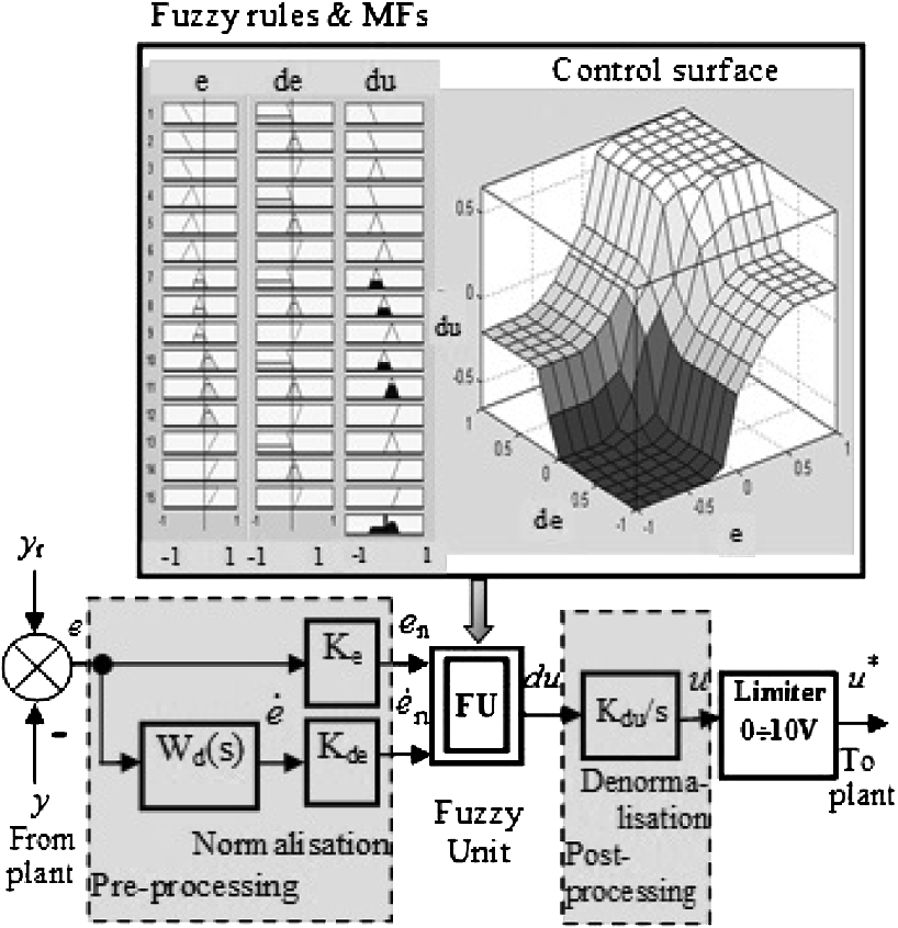
Fig. 2
Incremental PI-2I FLC with FU membership functions, fuzzy rules and control surface.
The designed PI-2I FLC is used in real time control of the air temperature. The temperature step responses to various reference changes from different operation points and the corresponding control is shown in Fig.
3 and further used in the TSK plant modelling and the NFPP training. The experiments are planned with respect to references and disturbances that ensure measurement data for the plant output
${y_{i}}$ in the whole range of its operation. The data should also be rich in magnitudes and frequencies to best reflect the system nonlinearity. They are split into a part
$({u_{k}^{1}},{y_{k}^{1}})$ (
$2/3$ of all data) used for the TSK plant modelling and the NFPP training, and a part
$({u_{k}^{2}},{y_{k}^{2}})$ for validation of the TSK model and the NFPP. The data samples
$({u_{k}^{1}},{y_{k}^{1}})$ are first pre-processed. Noise is filtered by smoothing. Correlation and size are reduced by dilution in time – the dilution sample time is
$k\Delta t$, where
$k=4\div 10$ is chosen to preserve the data pattern. Non-informative measurements are neglected. The data are also standardized or normalized in the range
$[-1,1]$ or
$[0,1]$. The pre-processed data is denoted as
$({u_{kn}^{1}},{y_{kn}^{1}})$.
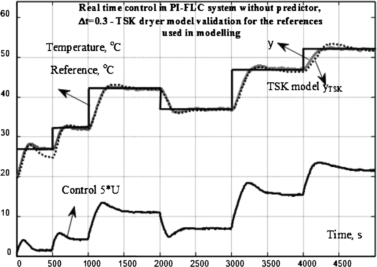
Fig. 3
Step responses of temperature and control action from real time PI-2I FLC plant control.
The standard TSK plant model consists of a FU with defined usually by experts N linear zones as input MFs. The input(s) z are measured or computed on the basis of measured variable(s). The current z is mapped into the MFs values ${\mu _{j}}$ $(j=1\div N)$ of belonging to the defined zones. The conclusions of the N fuzzy rules contain state space local linear dynamic models that describe the plant behaviour in the different operation zones. The TSK model output y is computed as a soft fuzzy blending (e.g. weighted average) of the current local plants outputs – $y={\textstyle\sum _{j=1}^{N}}{\mu _{j}}{y_{j}}/{\textstyle\sum _{j=1}^{N}}{\mu _{j}}$.
In the present research a modified TSK plant model is suggested and shown in Fig.
4 for
$N=3$ and
$z=y$. It consists of a zero order Sugeno Model and a separate dynamic part. The Sugeno Model is built of a FU with input
y and
N outputs with singletons as MFs and fuzzy rules that yield outputs equal to
${\mu _{j}}$. The FU input MFs like in the standard TSK model map the linear ranges (zones) according to expert information and are orthogonal, standard, defined in absolute universes of discourse. In Fig.
4 they are defined as
S for small
y,
M for medium
y, corresponding to the nominal linear operation zone, and
B for big
y. The dynamic part is based on transfer functions with easily estimated by experts type. It consists of
N parallel local linear models with the plant input
$u(t)$ as input and outputs
${y_{j}}(t)$ which are scaled by
${\mu _{j}}$ in fuzzy blending to yield the TSK plant model defuzzyfied output (Yordanova,
2011; Yordanova and Sivchev,
2014). The linear plant model in the
j-th zone in Fig.
4 is described by the transfer function
${P_{j}}(s)={K_{j}}{[{T_{j}}{T_{j+3}}{s^{2}}+({T_{j}}+{T_{j+3}})s+1]^{-1}}$, which can reflect the behaviour of many linear inertial plants with time delay from the engineering practice.
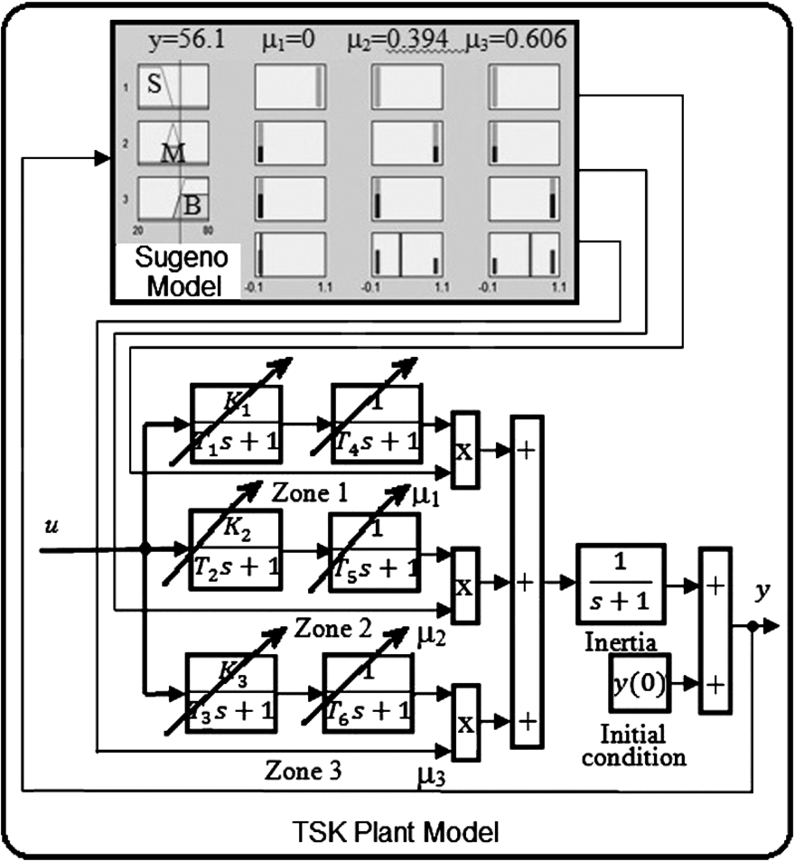
Fig. 4
Modified TSK plant model.
In general the parameters of the MFs and of the transfer functions of the local linear dynamic models in the modified TSK model can be computed via an optimization procedure for minimization of the modelling error. Here only the parameters
${\mathbf{q}_{\mathrm{TSK}}}=[{K_{1}},{T_{1}},{T_{4}};{K_{2}},{T_{2}},{T_{5}};{K_{3}},{T_{3}},{T_{6}}]$ of the local dynamic models in Fig.
4 are optimized by GAs minimization of the following fitness function:
where
$E(t)=y(t)-{y_{\mathrm{TSK}}}(t)$,
$y(t)$ is the plant output in Fig.
3 from the real time plant control and
${y_{\mathrm{TSK}}}(t)$ is the output of the TSK plant model in Fig.
4 from simulations of the closed loop system with the designed PI-2I FLC.
The GAs parameter optimization is based on a data sample of control action $U\in [0,4.7]$ and temperature y in the range between the ambient temperature $y(0)={19.7^{\circ }}$C and the maximal ${y_{\max }}={53^{\circ }}$C. The bounds for the tuning parameters ${\mathbf{q}_{\mathrm{TSK}}}$ are estimated on the basis of initial expert information about the plant.
The optimal parameters of the local linear plants computed are:
The reference step responses of the simulated system with the TSK plant model for
${\mathbf{q}_{\mathrm{TSK}}^{\circ }}$ ${y_{\mathrm{TSK}}}{^{(t)}}$ and the real plant output
$y(t)$ from the FLC real time temperature control are close as seen in Fig.
3.
The TSK plant model is ready for use and can ensure reliable results from simulations and system stability analysis after a successful validation. Therefore, the real time control system and the simulated system with the TSK plant model are subjected to reference changes different from the ones used in the TSK modelling. The step responses of the TSK plant model
${y_{\mathrm{TSK}}}(t)$ and the real plant
$y(t)$ are shown in Fig.
5. They are also close for
$y\leqslant 53$ and
$U\leqslant 4.7$ for which the TSK plant model is derived. This proves that the TSK plant model is adequate and accurate for all possible inputs in the defined ranges for
y and
U. In case the validation fails, a new GAs optimization should be started from different random values for the model parameters, changed bounds for them, or different GAs parameters – number of generations, mating and crossover method, mutation rate, etc.
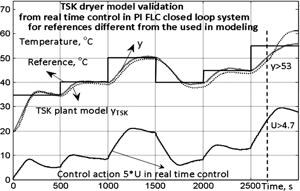
Fig. 5
TSK plant model validation for different references.
3 Design of a Neuro-Fuzzy Plant Predictor with Proper Prediction Horizon
The NFPP design, suggested here, consists of the following steps.
Step 1. Preparation of the training data. The training input–target couples
$[({u_{kn}^{1}},{y_{kn}^{1}}),{y_{kn+Hp}^{1}}]$ are obtained from the data
$(U,y)$ from PI-2I FLC real time plant control, shown in Fig.
3. The data is filtered from noise, normalized for
${U_{\max }}=4.7$ and
${y_{\max }}=53$ and with reduced correlation and size by taking every
kth element,
$k=4$. The training data sample period becomes
$4\Delta t=1.2$ s. The target vector with the predicted values
${y_{kn+Hp}^{1}}$ is computed from the input training sample
${y_{kn}^{1}}$ for an initial guess for the prediction horizon
${H_{p}}=10(4\Delta t)=12$ s in the estimated range of the plant time delay –
${H_{p}}\in [3,15]$ s.
The NFPP can be trained also on data from simulations of the closed loop system with the validated TSK plant model subjected to a great number of random in magnitude and duration reference changes in the operation range since simulation ensures fast responses, noiseless recorded data and full control over the simulation planned experiments. Thus, the dependence of the NFPP on the reference related training data is avoided.
Step 2. Design of a Sugeno NF model structure. Here a Sugeno NF model with three MFs for each input and singletons in the conclusions is assumed.
Step 3. NFPP training using ANFIS. The NFPP training ends successfully with the rules, the MFs and the prediction surface, presented in Fig.
6. The singletons in the conclusions are optimized to
$[0.37\hspace{0.2778em}0.61\hspace{0.2778em}0.97\hspace{0.2778em}0.46\hspace{0.2778em}0.69\hspace{0.2778em}0.97\hspace{0.2778em}00.73\hspace{0.2778em}1.02]$.
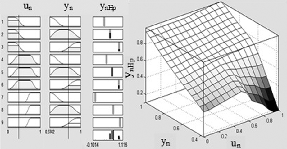
Fig. 6
Inputs membership functions, output singletons and fuzzy rules (left) and prediction surface (right) of the trained NFPP.
Step 4. Validation of the trained NFPP. The trained NFPP is validated for $[({u_{i}^{2}},{y_{i}^{2}})-{y_{i+{H_{p}}}^{2}}]$, obtained from the FLC real time plant control for different reference changes and disturbances from the ones used in the NFPP training. The aim is to prove that the NFPP has learned to correctly predict for all possible inputs in the defined ranges. The designed Sugeno NFPP in simulations has to respond to the inputs $({u_{i}^{2}},{y_{i}^{2}})$ with output close to the desired ${y_{i+{H_{p}}}^{2}}$.
The validation of the trained NFPP can be carried out also in real time control by feeding the predictor with the control signal and the output of the plant and comparing the delayed by time ${H_{p}}$ NFPP output with the plant output. The TSK plant model can be validated in a similar way of parallel operation – feeding the model with the real time plant input (the control action) and comparing the TSK model output with the plant output. The real time control of the plant has to use different reference changes and smaller sample period.
Here, the validation is carried out in two ways. The first one uses all the data
$(U,y)$ from the FLC real time control with
$dt=0.3$ s, but for new references. The obtained accuracy of prediction is high. The second one uses validation data, collected from the simulated FLC closed loop system with the TSK plant model for step reference changes with random magnitudes and duration. The normalized input data are applied to the NFPP and the denormalized predictor’s output
${y_{{H_{p}}}}$, delayed by the prediction time of 12 s, is compared with the TSK model output
${y_{\mathrm{TSK}}}$. The NFPP validation results in Fig.
7 show that the prediction of the trained NFPP is accurate for all possible inputs in the defined ranges and is independent of the references.
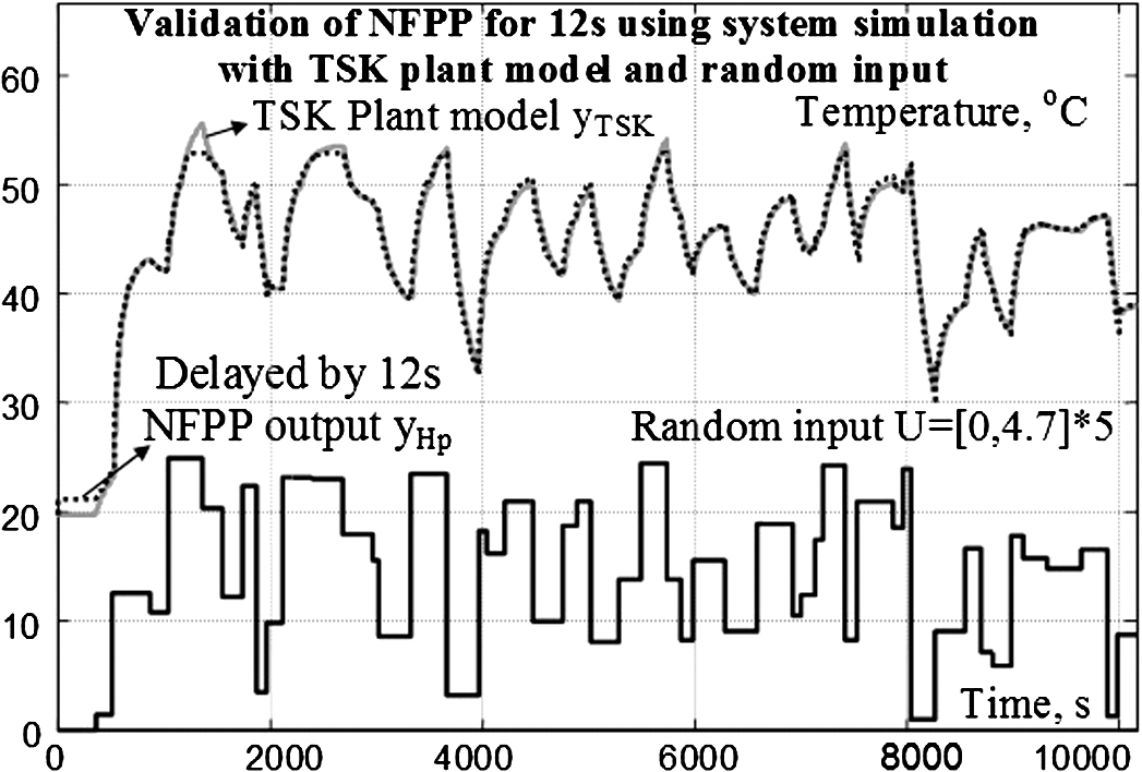
Fig. 7
NFPP validation with simulation data and random input.
If the validation is not successful – re-training from different random initial parameters or for a changed NF model (MFs number and shape, conclusions functions – singletons or linear type, etc.) is required.
The validated NFPP is implemented further in simulations and real time control with the necessary scaling factors (gains) for the normalization (standardization) of its inputs and the denormalization of its output.
Step 5. Selection of a proper prediction horizon. The accepted ${H_{p}}$ is proper when it ensures maximal improvement of the FLC-NFPP system performance with respect to the FLC system performance. This is assessed via simulation investigations of the FLC and the FLC-NFPP systems. For small improvement due to the NFPP the ${H_{p}}$ should be increased in the estimated range of the plant time delay. For too great ${H_{p}}$ a steady state error appears because the NFPP predicts the plant output far ahead when it is already equal to the reference which cheats the controller with a zero system error to keep the control action unchanged, while the real plant output differs from the reference. In both cases the NFPP needs to be re-trained and validated for the new ${H_{p}}$.
The simulated step responses of the closed loop systems with the TSK plant model and the designed PI-2I FLC and PI-2I FLC-NFPP for
${H_{p}}=12$ s are shown in Fig.
8. The performance of the PI-FLC-NFPP system is improved – the settling time, the overshoot and the control effort are reduced, and also there is no steady state error. So, the selected
${H_{p}}$ for the designed NFPP is suitable.
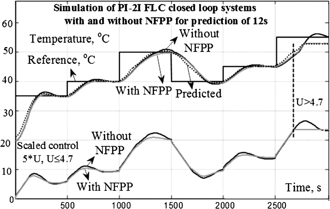
Fig. 8
PI-2I FLC and PI-NFPC systems investigation via simulation for determination of a proper ${H_{p}}$.
4 Study of the FLC-NFPP Closed Loop System Stability
The system stability analysis is based on the derived in Tanaka and Wang (
2001), Yordanova (
2011) Lyapunov conditions and their corresponding LMIs for a TSK-PDC system description.
Therefore, first the TSK-FLC-NFPP system has to be equivalently transformed into a TSK-PDC system by the design of a PDC that approximates the FLC-NFPP (NFPC). The PDC model structure is determined by the TSK plant model – the premises in the fuzzy rules are the same. The conclusions describe local linear controllers of selected algorithm. Their initial parameters are computed using empirical tuning methods to ensure stability and desired performance of the local closed loop systems. The final PDC nonlinear control is a fuzzy blending of the individual rules control actions.
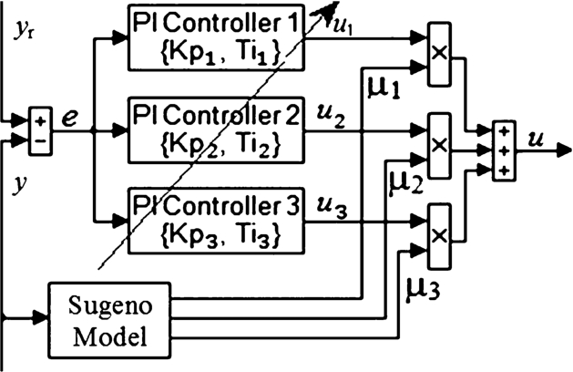
For the modified TSK plant model in Fig.
4 a corresponding modified PDC with local PI linear controllers with transfer functions
${C_{j}}(s)={K_{pj}}(1+1/{T_{Ij}}.s)$, shown in Fig.
9, is designed. The parameters of the local linear controllers are off-line GAs optimized via simulation of the NFPC and the PDC closed loop systems with the validated TSK plant model for the same input references, which change stepwise at random time moments with random magnitudes covering the whole range of operation. The accepted fitness function represents the relative integral squared error between the outputs
${y_{\mathrm{NFPC}}}(t)$ and
${y_{\mathrm{PDC}}}(t)$ of the simulated PI-2I FLC-NFPP (NFPC) and PI-PDC closed loop systems:
The computed optimal local PI controllers’ parameters ${\mathbf{q}_{\mathrm{PDC}}}=[{K_{p1}}=0.04,{K_{I1}}=0.001;{K_{p2}}=0.05,{K_{I2}}=0.0011;{K_{p3}}=0.06,{K_{I3}}=0.0013]$, where ${K_{Ij}}(s)={K_{pj}}/{T_{ij}}$, ensure ${F_{\mathrm{PDCmin}}}=0.5$, relative error $\mathbf{RE}=({y_{\mathrm{NFPC}}}-{y_{\mathrm{PDC}}})/{y_{\mathrm{NFPC}}}$ in the range of $\pm 4\% $, and accumulated absolute error $\textstyle\sum \mathrm{abs}(\mathbf{RE})=37$.
The designed PDC is validated via simulations of the PDC and the FLC-NFPP systems for smaller sample period and different reference changes than the ones used in the PDC design. The step responses of the original PI-NFPC and the PI-PDC systems for the new references are presented in Fig.
10, where
RE until
$U<4.7$ is bigger only at the beginning and
$\textstyle\sum \mathrm{abs}(\mathbf{RE})=39$ if the first step response is neglected. This shows a good PI-PDC approximation of the PI-NFPC. If the relative difference between the outputs of the two systems is not acceptably small, the PDC is re-designed with changed GAs parameters or types of local controllers.
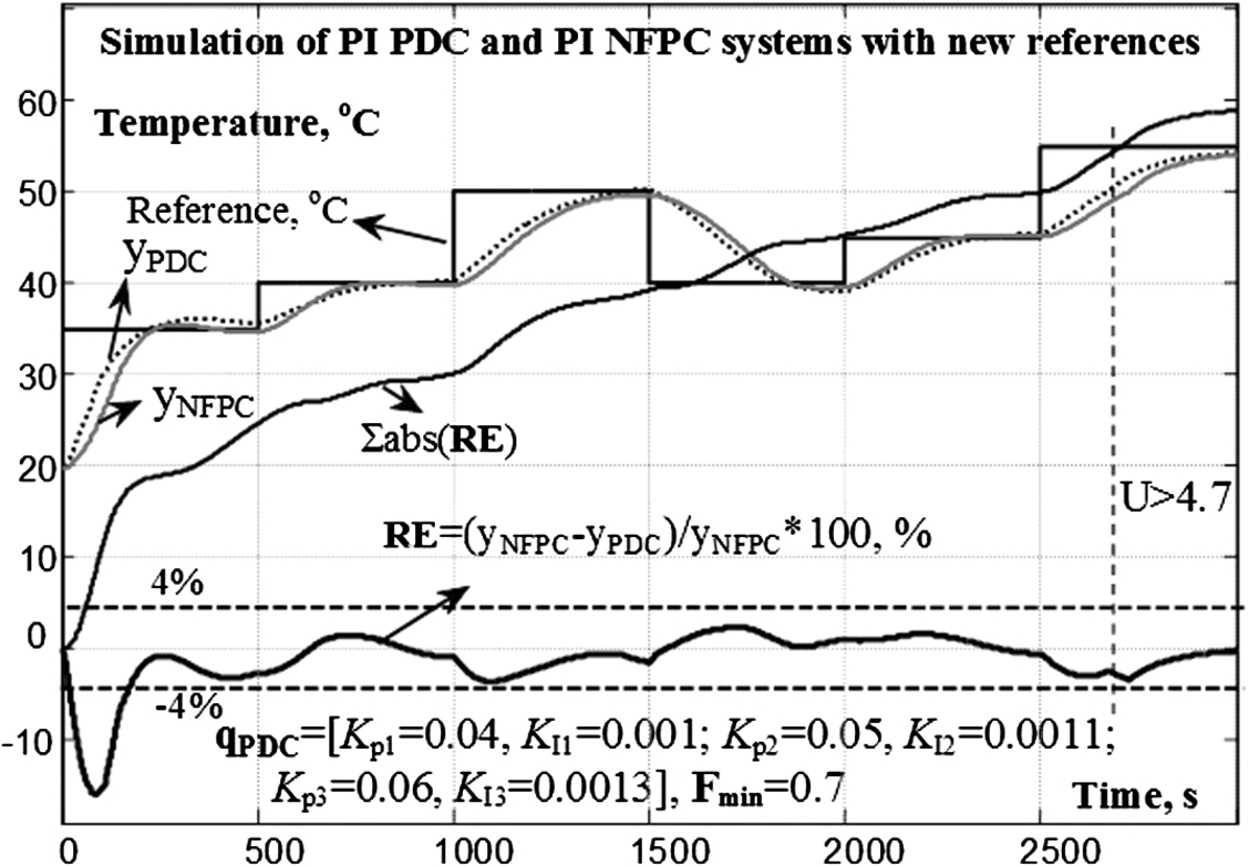
Fig. 10
Simulation of PI-PDC and PI-NFPC systems with new references for PI-PDC validation.
Then the modified TSK plant model and the modified PDC equivalent of the NFPC have to be presented into the standard state space description of the linear local plant models and controllers respectively in the fuzzy rules conclusions.
The TSK-PDC system stability analysis is of crucial importance since the system is nonlinear and operates with prediction, and the PDC is designed as a functional equivalent of the NFPC and not from local systems stability criteria.
So, first the local linear systems stability is studied applying linear control theory methods and if the stability is not ensured, the NFPP is re-designed for a smaller prediction horizon. Then the global nonlinear closed loop system stability is analysed using the Lyapunov stability conditions for a standard TSK-PDC representation of the plant and the controller (Tanaka and Wang,
2001):
where:
-
– $j=1\div N$ is the rule number;
-
– ${z_{px1}}$ is the vector of the premise variables with linguistic values $Lz$, defining the zones of the local linear plant models;
-
– ${x_{nx1}}$ is the state vector, ${y_{mx1}}$ – the output vector, ${u_{dx1}}$ – the input control vector and ${\mathbf{A}_{n\times n}}$, ${\mathbf{B}_{n\times d}}$, ${\mathbf{C}_{m\times n}}$ and ${\mathbf{D}_{m\times n}}$ – the corresponding matrices;
-
– $u=-\mathbf{F}x$ is a state feedback local linear controller for each local plant.
The Lyapunov sufficient condition for the closed loop system (3) to be globally asymptotically stable is the existence of a common for all local linear systems positive definite matrix
$\mathbf{P}>0$, such that the following matrix inequalities are satisfied for
$i,j=1\div N$,
$j>i$ and rule firing weights
${h_{i}}\cap {h_{j}}\ne \varnothing $ (Tanaka and Wang,
2001; Yordanova,
2011):
The conditions (
4) are transformed to the corresponding LMIs to be numerically solved as an optimization problem of the mathematical programming under convex restrictions (Balas
et al.,
2005; Tanaka and Wang,
2001). If solution exists, the system is stable, if not – it may be stable or not. Therefore, the FLC-NFPP has to be re-designed for new initial data, MFs, rules, FLC,
${H_{p}}$, data samples or TSK plant model and PDC.
Here the modified stability conditions (
4) in Yordanova (
2011,
2012) for other types of linear local controllers – dynamic compensators, PID, Smith predictor, etc. and for local linear plants with time delay are used.
The local PI controllers with output control action
${u_{j}}(t)={K_{pj}}e(t)+{K_{Ij}}\textstyle\int e(t)\hspace{0.1667em}dt$ are first turned into incremental PI controllers
${\dot{u}_{j}}(t)={K_{pj}}\dot{e}(t)+{K_{Ij}}e(t)$ and the integrators are equivalently added to the local linear plant models whose transfer functions become
${P_{j}}(s)/s$. Then the standard TSK-PDC description of the TSK plant and the PDC becomes:
where:
The Lyapunov stability condition for the specific TSK plant and PDC description (5) is solved using the corresponding LMIs for (4), and $-\mathbf{P}<-\mathbf{O}$. Since the open loop system is critically stable due to the integrator of the PI-PDC, instead of a zero matrix, O is chosen a matrix of ones in order to make the stability conditions more conservative with respect to finding a positive definite solution for the matrix P.
The computed for the investigated case study matrix
P is positive definite – all diagonal minors and
P have positive determinants, which proves the closed loop system stability:
The condition number $\mathrm{cond}(\mathbf{P})$ is small which guarantees low sensitivity to parameter variations, inaccurate data, computational and approximation errors.