Abstract
The present research shows the implementation of a virtual sensor for fault detection with the feature of recovering data. The proposal was implemented over a bicomponent mixing machine used for the wind generator blades manufacture based on carbon fiber. The virtual sensor is necessary due to permanent problems with wrong sensor measurements. The solution proposed uses an intelligent model able to predict the sensor measurements, which are compared with the measured value. If this value belongs to a specified range, it is valid. Otherwise, the prediction replaces the read value. The process fault detection feature has been added to the proposal, based on consecutive erroneous readings, obtaining satisfactory results.
1 Introduction
Not long ago, the majority of industrial activities were focused on increasing productivity and putting new processes and systems in operation. Regardless of the kind of application, system optimization has become a common goal. One of the reasons for this is the increasing competitiveness in every field Parmee and Hajela (
2012). To become more competitive, industries tend to decrease the consumption of energy in their productive processes, reduce environmental impact, minimize product failures, increase the general quality… In short, the optimization of production processes with minimum consumption and environmental impact has become a current goal for industries (Nicholson,
2017). Any contribution, no matter how small, can help achieve this objective.
One of the biggest problems experienced in the production process is the different anomalies that may occur during plant operation. They contribute to process failures and, consequently, to the deterioration of the overall quality of a product or a service. Usually, one of the typical problems that gives rise to these operating anomalies are inaccurate readings produced by malfunctioning sensors and transducers. This issue may seem to be a minor problem. However, when a process relies on the values read, the consequences of using incorrect values can be very critical (Sharma
et al.,
2010).
In Wang and Cui (
2005), two different kinds of errors in sensors are described: complete failure and bias error. The first case is relatively easy to solve. However, the second one requires close attention, even failure detection is not easy to identify. From the point of view of an operating plant, bias failures could entail problems in terms of control, Fault Detection and Diagnosis (FDD), optimization, and of course, plant monitoring.
With the aim of preventing sensor failures and, consequently, the above mentioned problems, one of the common methods consists in the implementation of physical redundancy, for both fault detection and accomplishment of diagnosis tasks (Hwang
et al.,
2010). In some critical applications, like nuclear energy plants, the use of this kind of redundancy is very common. However, the use of this method has been reduced significantly in the last years due to its high cost and complexity implementation, among other reasons (Wang and Cui,
2005).
A suitable alternative, used especially in applications that are not very critical, consists in using virtual sensors for failure detection. Besides, this alternative could be applied as a complementary tool for critical applications.
With this method, it is possible to detect both errors, complete failure and bias deviation. When a sensor reads a value incorrectly, it will be possible to estimate the percentage of its error if necessary (Naidu
et al.,
1990). There are some proposals where an algorithm is created to accomplish fault detection and, when there is a fault, it is isolated and recovered (Carvajal-Godinez
et al.,
2017).
Due to the rise in popularity of automated processes, it is necessary to measure a huge quantity of variables to fulfil different tasks, such as monitoring or control. To accomplish this goal successfully, the correct functioning of all sensors of the system is mandatory. This is not an easy task, because normally sensors operating in industrial environments (Shen
et al.,
2015) experience some failures. In a typical process, it is possible for one or more of those anomalies to occur: faults in actuators, disturbances in the process, sensor faults and measurement noise (Carvajal-Godinez
et al.,
2017). With the aim of mitigating the above mentioned possibilities, it would be necessary to develop an algorithm for fault detection which would isolate the errors in its first step and then would recover the correct data (Heredia and Ollero,
2010).
This work addresses the problem of an automatic mixing machine for obtaining a bicomponent product used in the manufacture of wind generator blades, whose primary element is carbon fiber. In this case specifically, the mixture consists of two products, the first one is an epoxy resin, and the second one is a catalyst. If the proportions of those two products are correct and stable in the mixture, the product acquires the desired properties. This process is very difficult to control due to the Non-Newtonian nature of the primary components, because their properties depend on the fluid stress (Fan
et al.,
2006). Also, the system is located in an industrial environment and is therefore affected by all the sensor-related problems. Thus, the implementation of a virtual sensor is proposed for fault detection, error isolation and recovery of the correct data. Furthermore, the algorithm should be able to detect sensor and process failures when they provide inaccurate readings consecutively.
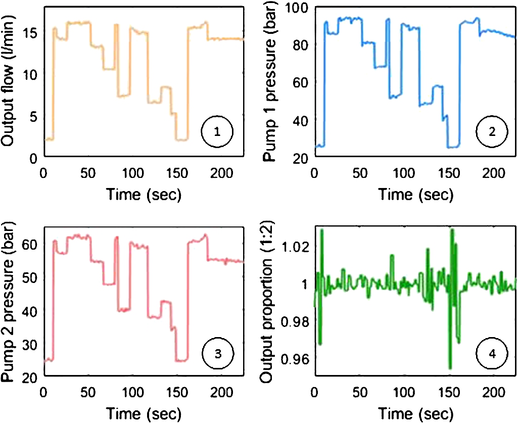
Fig. 1
Variables measured during system operation.
The structure of this work is organized as follows. After the present section, the next section describes the system, the existing variables, and provides a brief introduction to the virtual sensor developed to detect the incorrect readings and system failures. Then, the implemented model and the applied algorithms are shown. After that section, the results obtained with the implementation of this novel model are presented. Finally, the conclusions and the possible future lines of research are listed.
2 Case Study
2.1 Bicomponent Mixing System
Prior to sensor modelling, an initial description of the installation under study is developed in this section. The wind generator blades are manufactured using the bicomponent material obtained at the output of the mixing machine installation. This material is the result of mixing two different fluids (Fluid 1 and Fluid 2), which are initially stored in separated tanks. The fluids are pumped by two gear pumps, which are coupled to electric engines actuated by two variable frequency drives that follow the control signals provided by the controller. The two pumped fluids are mixed through a mixing valve which gives the necessary objective material throughout the wind generator blade.
The graphs shown in Fig.
1 represent an example with the values of different system variables during the blade manufacture. As the blade shape is not uniform, the output flow rate is not constant (1). Hence, the pressures of pumps 1 and 2 change depending on the part to be manufactured (2, 3). These variations lead to fluctuations in the product proportion of the final mixed product (4).
To achieve a representative model, all the operating ranges of the installation must be taken into account.
2.2 Variables Monitored
For each operating range, all the values measured by the sensors located along the installation were recorded during its normal operation. This is a key step in the implementation of the virtual sensor. This research uses a dataset that consists of different plant parameters measured during normal system operation.
Three flowmeters are located in the different pipelines of the mixing machine. They measure the flows of Fluid 1, Fluid 2 and the final material, in liters per minute (Flow 1, Flow 2, Output Flow). Also, four pressure sensors are used to monitor the pressure (bar) along the circuit. Two of them are located behind each pump (Pump 1 pressure, Pump 2 pressure) and the other two sensors are deployed behind the flowmeters of lines 1 and 2 (Flowmeter 1 pressure, Flowmeter 2 pressure).
A part from the measured variables, there are some system variables that are recorded. These monitored variables are the desired and the real proportions of materials 1 and 2 (Proportion Set Point, Output Proportion) and also the speeds of both pumps 1 and 2 (Pump speed 1, Pump speed 2), in rpm.
The diagram shown in Fig.
2 represents the sensors located in the mixing machine installation.
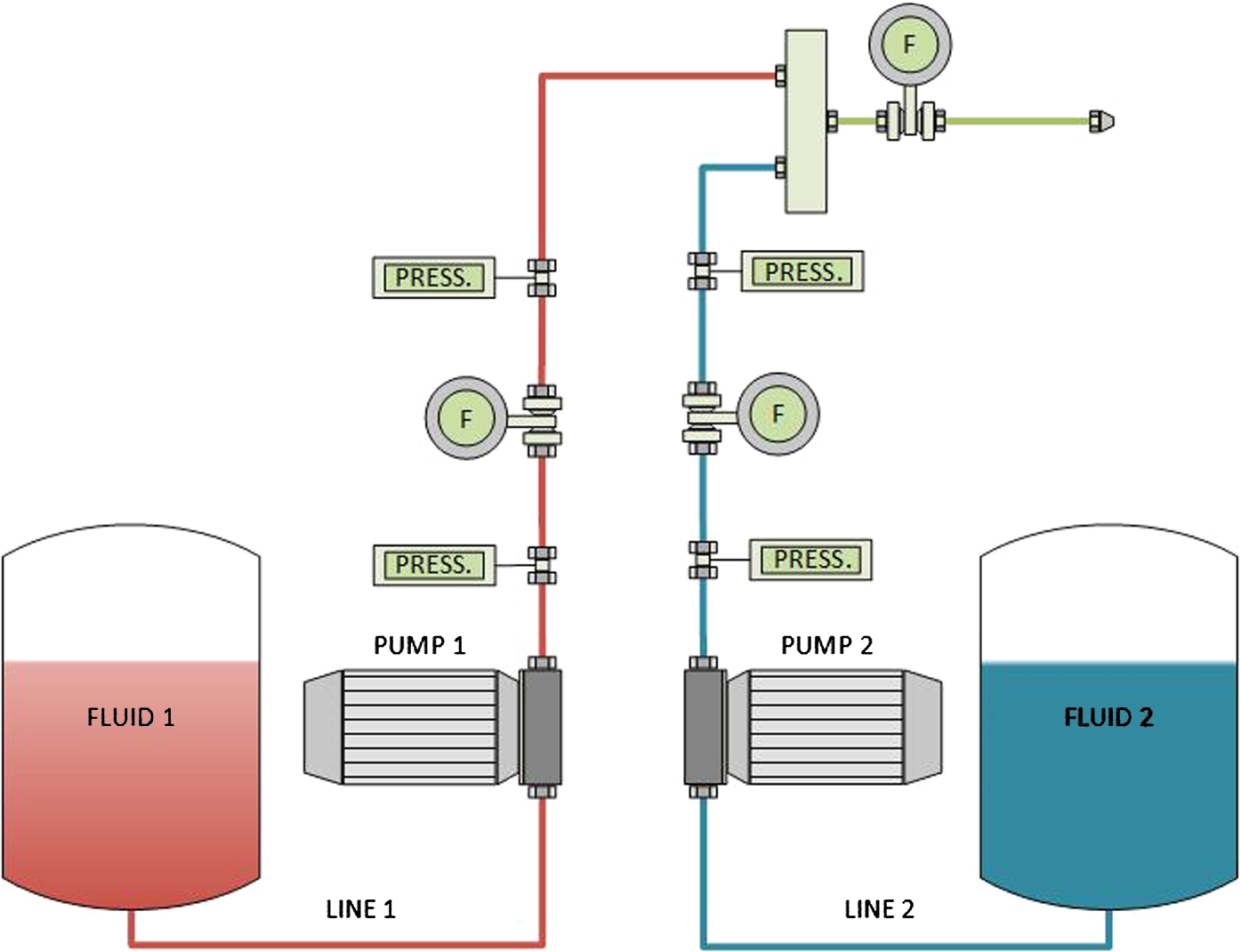
Fig. 2
Bicomponent mixing system scheme.
2.3 Virtual Sensor Implementation
Some failures might occur during the mixing process. Figure
3 shows the measured
Output Flow with missing values due to a sensor failure.
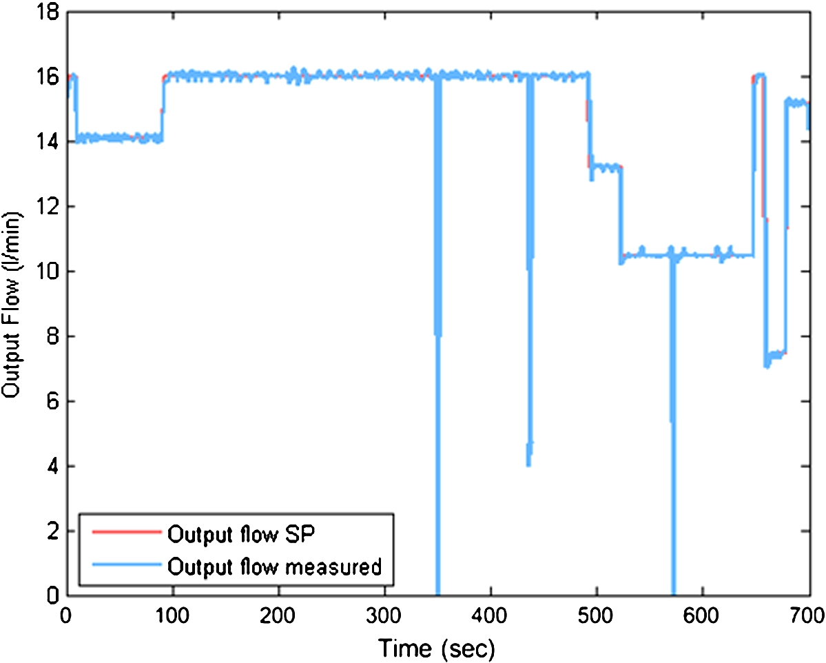
Fig. 3
An example of the output flow with erroneous measurements.
This research aims to design a virtual sensor that ensures that only the correct values are used in processes by replacing erroneous measurements values with the output values given by the model. Moreover, if the measurement of the real sensor is different from the predicted value in some samples, the virtual sensor should detect a failure in the system. A failure can have two possible sources, either a sensor or the system. Since the model is trained with data from correct system operation, the values that deviate considerably from the predicted ones indicate that the system is not functioning properly.
3 Soft Computing Techniques
The soft computing techniques used to create our novel hybrid system are described in detail below.
3.1 K-means Algorithm. Data Clustering
Clustering, a key unsupervised learning algorithm (Kaski
et al.,
2005), consists in the process of distributing different data into groups that have a common feature. A cluster is defined as a set of objects that present similarity between them and have different features than the ones located in other clusters (Qin and Suganthan,
2005; Ye and Xiong,
2007).
Among the great variety of cluster algorithms, they can be divided into agglomerative hierarchical clustering methods and iterative square-error partitional clustering methods (Pal and Biswas,
1997).
Partitional clustering algorithms split the initial dataset into a number of clusters specified by the user, minimizing specific criteria. Agglomerative clustering algorithms begin by agglomerating all the data in a singleton cluster and then, nearby clusters are united. When the stop criteria are reached, the clustering is completed.
The commonly used
K-means (Jain,
2010) is a clustering algorithm based on two input arguments: the number of clusters
K into which the dataset will be divided and the centroid location of each cluster. The training process consists in assigning each data sample to the nearest group centroid. When the groups are formed, the centroids’ locations are recalculated. This procedure is repeated until no changes are produced in all centroids. The use of
K-means leads to successful results, especially when clusters are hyperspherical and separated enough in the hyperspace (Garg
et al.,
2011).
3.2 Artificial Neural Networks (ANN). Multilayer Perceptron (MLP)
An artificial neural network (ANN) is a system designed to emulate the specific brain operations. In the last years, ANN have been applied successfully to solve real and challenging problems (Wasserman,
1993; Zeng and Wang,
2010; González
et al.,
2015; Pinzón
et al.,
2010; Sánchez
et al.,
2013). One of the most used supervised learning ANN is the Multilayer Perceptron (MLP) due to its simple structure and robustness (Wasserman,
1993; Zeng and Wang,
2010). It has one input layer, one output layer and one or more hidden layers. These layers are made of neurons and weighted connections link different layer neurons. The weights of each connection are tuned to decrease the error if the output of the network does not coincide with a known target output. Despite the simplicity of its architecture, the ANN parameter must be chosen properly in order to achieve satisfactory results. In the most common configuration, the same activation function is assigned to all neurons in a layer. The activation function can be linear, step, tan-sigmoid or log-sigmoid.
In this work, the MLP-ANN algorithm used for regression is composed by only one hidden layer and the number of neurons is tested from 1 to 15. The activation functions are tan-sigmoid at the hidden layer neurons and linear at the output.
The employed learning algorithm was Gradient descent, and the algorithm for model training was Levenberg-Marquardt. Also, to measure the network performance, the MSE (Mean Squared Error) method was applied.
3.3 Support Vector Regression (SVR), Least Square Support Vector Regression (LS SVR)
The support vector machine (SVM) is a supervised form of machine learning that is normally used in classification problems (Rebentrost
et al.,
2014; Qi
et al.,
2013). However, it is also used in regression tasks (Fei and Bai,
2014; Hu
et al.,
2014).
For binary classification problems, the aim of SVM is to design a hyperplane for the classification of all the training data into two classes by finding the maximum distance between the locations of the closest data points of both classes and the hyperplane. The training instances presented near the hyperplane are defined as support vectors. Therefore, SVMs perform the projection of the training dataset in a high dimensional feature space using a kernel operator.
SVM can also be used for regression (SVR) by performing minor changes in the original algorithm used for classification problems. The SVR represents the initial dataset in terms of a multi-dimensional feature space
F using a non-linear mapping and then, linear regression in
F (Cristianini and Shawe-Taylor,
2000; Steinwart and Christmann,
2008).
Least Square formulations of the SVM are known as LS SVM. This technique obtains the solution by solving a linear equations system, which, in terms of performance and generalization, is similar to SVM (Suykens and Vandewalle,
1999; Wang
et al.,
2012). LS SVR is defined as the application of LS SVM to regression (Guo
et al.,
2012; Wang and Wu,
2012). In this case, a squared loss function replaces the insensitive loss function.
In this paper, the KULeuven-ESAT-SCD self-tuning was implemented. The selected parameters were ’Function Estimation’ to conduct the regression and Radial Basis Function (RBF) for the model kernel. The used cost criteria was ’leaveoneoutlssvm’ with ’mse’ and the optimization function was configured as ’simplex’.
4 Model Approach
This section describes the different blocks used to obtain the virtual sensor developed in this paper.
4.1 Hybrid Intelligent Models
The first step in the development of a virtual sensor capable of detecting anomalies in the plant under study, consists of using intelligent regression techniques combined with clustering algorithms. In the specific case explained in this paper, the real sensor under study, whose measurements are predicted, is the Flow 1. Then, the signals used to obtain the regressive models are: Output Flow, Flow 2, Pump 1 pressure, Pump 2 pressure, Flowmeter 1 pressure and Flowmeter 2 pressure. Also, the two previous states of each signal are taken into account, including the previous states of Flow 1, the output of the model.
As the dataset may consist of data with different behaviours, clustering algorithms are applied to group them accordingly. Then, the hybrid intelligent model used in this research is based on local models in order to increase the global performance of the predicted signal. This means that, for each cluster, a new model is obtained by using the intelligent regression techniques.
Figure
4 represents the hybrid model internally, with the connections to the fault detection block presented in next subsection. The cluster selector block (Fig.
4) is used to internally assign the input data to its cluster according to its nature. The specific model of that cluster is used to predict the output. When the sensor signal is predicted, it is routed to the fault detection block.
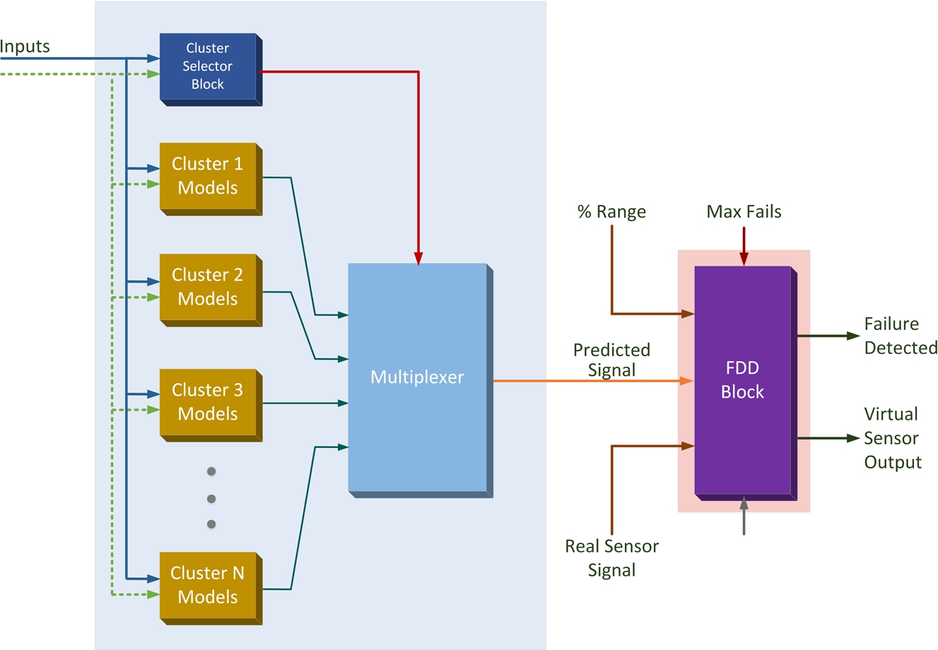
Fig. 4
Failure detection and virtual sensor diagram.
4.2 Model Selection
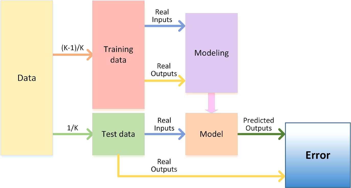
Fig. 5
Modelling process.
To achieve the best model performance, Global and Local models have been considered. As a hybrid model consists of some clusters, the global model is the one that only has one cluster division. Once the data is divided into different clusters using the
K-means algorithm, the described regression techniques are applied to each group. In all cases (Global and Local models), the
k-fold modelling process is shown in Fig.
5, and follows the subsequent steps:
-
• Given a specific value of K, the dataset (which consists of the whole data or the data of just one cluster) is divided into two different groups: training and test data.
-
• Model training: an intelligent model with the regression techniques described in Sections
3.2 and
3.3 (MLP and LS SVR) is implemented. The training data, composed by
$(1-K)/K$ samples, is used to train an intelligent model.
-
• Model test: once the model is obtained, its performance is checked using the test data, composed by $1/K$ samples that are used as inputs of the trained model.
-
• The outputs predicted by the model are compared with the real outputs and then, the error is calculated.
To achieve a better generalization and a more real model performance, the content of training data and test data are shifted as shown in Fig.
6 (Bishop,
2006). Hence, for a specific regression technique with a
$K=10$, ten different models are created. Then, an averaged Mean Squared Error (MSE) is calculated from the results of each of the ten models.
Therefore, the process shown in Fig.
5 and Fig.
6 is followed to assess the performance of different techniques. The criteria for the selection of the best technique is based on the lowest MSE. As explained before, the
k-
fold can be applied over one cluster when the
K-
means algorithm is used, or it can be applied over the complete dataset to obtain a global model.
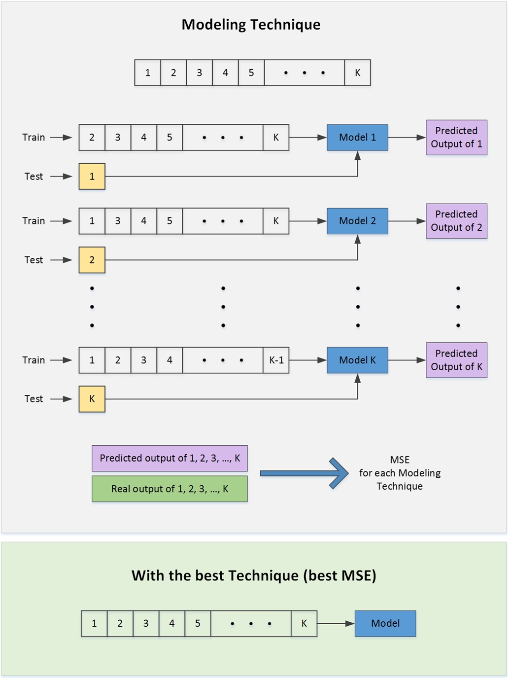
Fig. 6
K-Fold performance calculation.
4.3 Fault Detection Block
Once the hybrid intelligent model predicts the measurement of the sensor, the model approach for the virtual sensor is presented in Fig.
7.
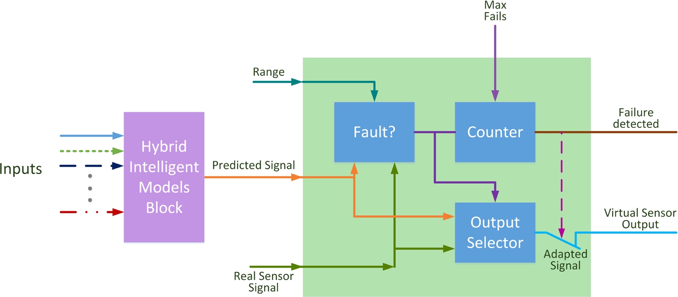
Fig. 7
Proposal of the virtual sensor model.
The fault detection algorithm is applied according to the green block in Fig.
7. For greater clarity, the figure includes a description of the workflow of this block. The real and the predicted signals are compared and the maximum error allowed between the two values is defined by
Range signal, a virtual sensor input. If the real signal fits within the specified range, the output of the virtual sensor will be the same as the real value measured by the sensor. If this is not the case, the predicted signal will be used. The fault detection algorithm only allows this fault situation for several consecutive samples. The maximum number of failures allowed is defined by the input signal “
Max.Fails”. If the number of consecutive failures exceeds the number of failures defined by this input, the
Failure detected signal is set, and the output of the virtual sensor is turned off. The specific configuration in
Range and
Max.Fails depends on the sensor and the system in which the virtual sensor is implemented.
The proposed FDD system is designed to allow for a maximum of 5 inaccurate measurements in consecutive order before the fault detection alarm is set. These 5 samples allow the system to filter incorrect measurements like the ones shown in Fig.
3, and also make it possible to detect a failure in the sensor. It is necessary to remark that, when a failure is detected, it might not be caused by a fault in the sensor, it could be a system failure. In such cases, all the sensors take inaccurate measurements and the model does not predict correct values. In this situation, the detection system is unable to recognize if the incorrect signal is caused by the sensor under supervision or by the predicted signal.
If the rest of the sensors (the model inputs) have incorrect values, a failure in the process could not be detected. However, if all the sensors have similar FDD system as the one described in this paper, an incorrect value in all FDD would mean a process failure.
4.4 Dataset Description
The dataset used in this research was created by means of many different tests carried out during the operating process.
The original dataset consisted of a total of 9511 samples. After the pre-processing, which consisted in removing the incorrect measurements, the final dataset used to generate the novel model contains 8549 samples, with the variables Output Flow, Flow 1, Flow 2, Pump 1 pressure, Pump 2 pressure, Flowmeter 1 pressure, Flowmeter 2 pressure.
5 Results
The predictive model is designed to take into account the last two measures of each sensor (six sensors and the predicted sensor value). This way, the model can reflect the system dynamics, achieving a better performance in the prediction. Therefore, the model has 20 inputs: the two previous values of Flow 1 and the values of the current and the two previous measures of the sensors Output Flow, Flow 2, Pump 1 pressure, Pump 2 pressure, Flowmeter 1 pressure and Flowmeter 1 pressure.
The model output represents the current prediction of value of the Flow 1 sensor. Different simulation tests were performed in order to check that these values are enough to learn system dynamics. Results demonstrate that including a higher input regression vector does not lead to an improvement in model accuracy.
A statistical analysis was conducted using a 10 K-fold cross-validation to obtain the MSE of each cluster model.
Once the model for each technique is obtained, the criteria for the choice of the best technique performance are based on the MSE. Table
1 represents the lowest MSE in the
Flow 1 prediction, depending on the number of clusters. For example, if the dataset is grouped in two clusters, the error obtained is 0.1856e−3 if the data belongs to cluster 1 and 0.1920e−3 if it belongs to cluster 2.
To assess the relationship between the number of clusters and the general performance of each cluster configuration, the mean MSE value is calculated (Table
2). This average MSE is obtained considering the number of samples at each cluster to ensure a representative measurement of each configuration. Then, Table
2 shows that dividing the data into 7 clusters leads to the best model performance.
| N° of clusters |
Cl. 1 |
Cl. 2 |
Cl. 3 |
Cl. 4 |
Cl. 5 |
| 1 |
0.1502e−3 |
– |
– |
– |
– |
| 2 |
0.1856e−3 |
0.1920e−3 |
– |
– |
– |
| 3 |
0.2001e−3 |
0.1654e−3 |
0.1338e−3 |
– |
– |
| 4 |
0.2108e−3 |
0.1191e−3 |
0.2119e−3 |
0.1312e−3 |
– |
| 5 |
0.2890e−3 |
0.0815e−3 |
0.2149e−3 |
0.1845e−3 |
0.0937e−3 |
| 6 |
0.1245e−3 |
0.1249e−3 |
0.2358e−3 |
0.0956e−3 |
0.1963e−3 |
| 7 |
0.1652e−3 |
0.1594e−3 |
0.0979e−3 |
0.0552e−3 |
0.1837e−3 |
| 8 |
0.1660e−3 |
0.3115e−3 |
0.1117e−3 |
0.1213e−3 |
0.2123e−3 |
| 9 |
0.1981e−3 |
0.1667e−3 |
0.4204e−3 |
0.0479e−3 |
0.1557e−3 |
| 10 |
0.1400e−3 |
0.1759e−3 |
0.1188e−3 |
0.3019e−3 |
0.1192e−3 |
| N° of clusters |
Cl. 6 |
Cl. 7 |
Cl. 8 |
Cl. 9 |
Cl. 10 |
| 1 |
– |
– |
– |
– |
– |
| 2 |
– |
– |
– |
– |
– |
| 3 |
– |
– |
– |
– |
– |
| 4 |
– |
– |
– |
– |
– |
| 5 |
– |
– |
– |
– |
– |
| 6 |
0.1464e−3 |
– |
– |
– |
– |
| 7 |
0.1637e−3 |
0.1221e−3 |
– |
– |
– |
| 8 |
0.2321e−3 |
0.1845e−3 |
0.0926e−3 |
– |
– |
| 9 |
0.1117e−3 |
0.0888e−3 |
0.2480e−3 |
0.1205e−3 |
– |
| 10 |
0.4108e−3 |
0.1912e−3 |
0.0983e−3 |
0.2047e−3 |
0.1222e−3 |
Table 2
Mean MSE for each model depending on the number of clusters.
| N° of |
Mean squared |
| clusters |
error |
| 1 |
0.1502e−3 |
| 2 |
0.1894e−3 |
| 3 |
0.1602e−3 |
| 4 |
0.1584e−3 |
| 5 |
0.1485e−3 |
| 6 |
0.1528e−3 |
| 7 |
0.1314e−3 |
| 8 |
0.1522e−3 |
| 9 |
0.1553e−3 |
| 10 |
0.1698e−3 |
As a hybrid model is proposed, the technique used to predict the measurements of
Flow 1 sensor depends on the cluster configuration. Table
3 summarizes the best regression technique for each cluster. Considering the example with two clusters, proposed in the previous paragraph, the sensor measurement is predicted using a neural network with 5 hidden layer neurons, if the input data belongs to cluster 1. Otherwise, a neural network with 8 hidden layer neurons would be used.
Table 3
Best regression technique for each cluster depending on the number of clusters.
| N° of clusters |
Cl. 1 |
Cl. 2 |
Cl. 3 |
Cl. 4 |
Cl. 5 |
| 1 |
ANN-11 |
– |
– |
– |
– |
| 2 |
ANN-5 |
ANN-8 |
– |
– |
– |
| 3 |
ANN-5 |
ANN-5 |
ANN-8 |
– |
– |
| 4 |
ANN-3 |
ANN-4 |
ANN-3 |
ANN-9 |
– |
| 5 |
ANN-1 |
ANN-4 |
ANN-1 |
ANN-8 |
ANN-8 |
| 6 |
ANN-1 |
ANN-7 |
ANN-4 |
ANN-6 |
ANN-3 |
| 7 |
ANN-1 |
ANN-1 |
ANN-7 |
ANN-5 |
ANN-3 |
| 8 |
LS SVR |
ANN-1 |
ANN-4 |
ANN-1 |
ANN-2 |
| 9 |
LS SVR |
ANN-1 |
LS SVR |
ANN-4 |
ANN-1 |
| 10 |
ANN-4 |
ANN-2 |
ANN-4 |
LS SVR |
ANN-1 |
| N° of clusters |
Cl. 6 |
Cl. 7 |
Cl. 8 |
Cl. 9 |
Cl. 10 |
| 1 |
– |
– |
– |
– |
– |
| 2 |
– |
– |
– |
– |
– |
| 3 |
– |
– |
– |
– |
– |
| 4 |
– |
– |
– |
– |
– |
| 5 |
– |
– |
– |
– |
– |
| 6 |
ANN-15 |
– |
– |
– |
– |
| 7 |
ANN-3 |
ANN-8 |
– |
– |
– |
| 8 |
ANN-2 |
ANN-3 |
ANN-10 |
– |
– |
| 9 |
ANN-10 |
ANN-4 |
ANN-1 |
ANN-13 |
– |
| 10 |
LS SVR |
ANN-2 |
ANN-5 |
ANN-4 |
ANN-7 |
Once the best model is chosen, the resulting hybrid intelligent model was implemented taking into account the best algorithm for each cluster.
Fault Detection System Results
To test the FDD system, two types of errors are simulated. In Fig.
8 it is possible to see the test data used by the system; in the upper side, the real value of the sensor is shown in a blue-continuous line. In the middle of the figure, the predicted output from the model is plotted in red-dash line; in the bottom side, the error signal is shown in a black-dotted line.
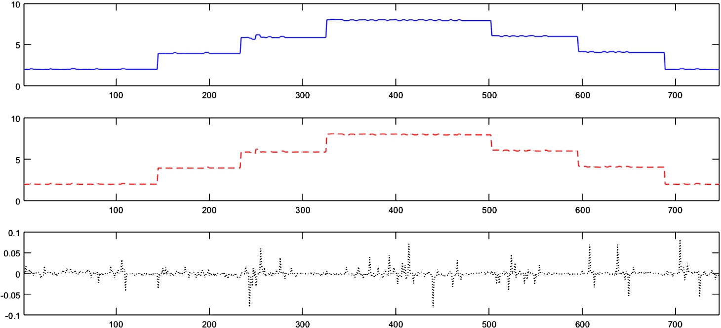
Fig. 8
Data to test the fault detection and diagnostic system.
To test the FDD system, some failures are introduced into the value data of real sensor. Figure
9 shows one of the tests performed. In this case, the graph on the top gives the real sensor values (blue continuous line), where the different simulated sensor failures can be observed. The tested failures are the most typical failures, such as the missing data or sensor saturation. Moreover, at the end of the plot, a failure in the sensor is simulated as a degradation in the measured value until it completely fails. The second plot (red dashed line) represents the values predicted according to the model. The previous values used as inputs are the output of the FDD system, not the sensor value. In case of detecting a measurement that is out of the defined range, the output will be the predicted value, and is the one used as previous value in the model. The third graph is the alarm situation signal, which is activated when the error signal is greater than the range set. However, the system continues working until more than 5 consecutive alarms are detected. The bottom of Fig.
9 is the output of the system, where it can be seen that the incorrect measurements were replaced by the predicted values, until the error samples had more than 5 errors in a row; that is when the system stops working.
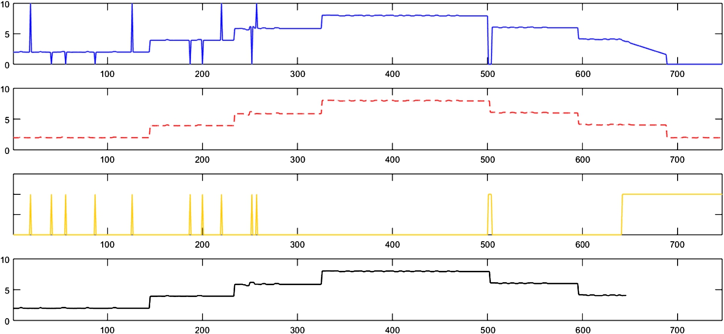
Fig. 9
Fault detection and diagnostic system simulation.
6 Conclusions
This paper has proposed a virtual sensor for fault detection, isolation and data recovery in a bicomponent mixing machine. The virtual sensor uses a hybrid intelligence model to predict the signal value in a specific sensor. In the described case, the catalyst flow sensor is studied. The model output is the predicted measurement of the sensor under study. The model inputs are the current value and last two values of the other sensors, and the last two states of the output.
Overall, all models are capable of predicting the readings of sensor Flow 1 with a maximum error of 0.1894e−3. The best performance is achieved when the dataset is grouped in 7 clusters, with a mean error of 0.1314e−3. Moreover, this hybrid model, which combines different intelligent techniques, proves to be a very good predictor of the current state of the sensor.
This feature plays a key role in the implementation of the FDD system by comparing the measured value with the predicted one. The method was validated in terms of three different kinds of failures; a missing measurement, sensor saturation and sensor degradation. In all cases, the system has been able to detect the failures and to replace the inaccurate data successfully.
The virtual sensor works by selecting between the real and the predicted measurement when failures are detected. The permitted range of deviation between the real and the predicted signal can be changed by user. Another input that can be adjusted is the maximum number of samples needed to detect a fault. The system allows for specific consecutive failures. When this signal alerts of a failure, the output of the virtual sensor is opened, because it could be necessary to check the sensor.
The use of the FDD system proposed in this work can be used as a very useful tool for the detection of anomalies on an industrial plant. Anomaly detection is a crucial step in the improvement of plant performance, maintenance planning, product quality, energy optimization, and more.