1 Introduction
HyperSpectral Images (HSIs) contain an exhaustive variety of information about specific characteristics of the materials, with hundreds or even thousands bands (Borengasser
et al.,
2007). The spectrum of each pixel can be seen as a vector, where each component represents the luminosity of the reflectance value for each spectral band. The set of bands which composes an HSI shows the representation of a scene, but each one individually contains information from a different wavelength range, which can cover both the visible and infrared spectrum. The width of each band can be between 5 and 10 nm, depending on the considered sensor. Each material throws a different reflectance profile for all the bands. Thus, for each point of the image, a specific curve that provides a lot of information for the corresponding point of the scene is obtained. Therefore, to efficiently exploit this information in applications, classification of HSIs is usually performed, where pixels are labelled to one of the classes based on their spectral characteristics.
There are many applications which take advantage of a large amount of information provided by hyperspectral sensors, such as remote sensing (Wang
et al.,
2017), biotechnology (Asaari
et al.,
2018), medical diagnose (Leavesley
et al.,
2018), forensic science (Almeida
et al.,
2017), environmental monitoring (Virlet
et al.,
2017), etc. This available information leads us to develop new processing techniques. In addition, many applications which work with HSIs require a fast response. Examples of these applications may be obtained in the areas of modelling and environmental assessment, detection of military objectives or prevention and response to risks, such as forest fires, rescue operations, floods or biological threats (Chang
et al.,
2001; Manolakis
et al.,
2003).
However, the large amount of information contained in an HSI, which is its main advantage, is also a disadvantage in terms of computational performance. The work with large HSIs involves a high computational complexity and requires a lot of resources and time (Rizzo
et al.,
2005). On the other hand, it is well-known that high-dimensional data spaces are mostly empty. This indicates that the data structure of an HSI exists basically in a subspace (Plaza
et al.,
2005). Taking into account these ideas, it can be concluded that there is a need (and a possibility) to reduce the size of the HSIs. So, it is usual to apply techniques to reduce the dimensions of the original HSIs, obtaining reduced images which can be handled in a more efficient way without losing critical information (Harsanyi and Chang,
1994; Bruce
et al.,
2002; Wang and Chang,
2006).
Multidimensional Scaling (MDS) consists of a set of techniques which are used to reduce the dimensions of a data set. Such techniques are used in many applications – multiobjective optimization (Filatovas
et al.,
2015), data mining (Medvedev
et al.,
2017), (Bernatavičienė
et al.,
2007), marketing (Green,
1975), cryptography (Gupta and Ray,
2015), a wide variety of mathematical and statistical methods (Granato and Ares,
2014), psychology (Rosenberg,
2014), etc. They use a mapping function usually based on Euclidean distances which is able to find an optimal data representation. However, also other distance metrics could be considered (Fletcher
et al.,
2014). MDS techniques represent data in a low-dimensional space in order to make these data more accessible (Borg and Groenen,
2005; Dzemyda
et al.,
2013). For instance, a graphical visualization of the data in
$2D$ or
$3D$ space for an easier understanding of the information.
A well-known technique named Isometric mapping (Isomap) generalizes MDS to non-linear manifolds, replacing Euclidean distances by geodesic distances (Bengio
et al.,
2004). Isomap has been used successfully in a multitude of applications, such as HSIs (Li
et al.,
2017), face recognition (Yang,
2002a), biomedical datasets (Lim
et al.,
2003), pattern classification (Yang,
2002b), learning multi-class manifold (Wu and Chan,
2004), supervised learning (Pulkkinen
et al.,
2011), etc. Focusing on the HSIs, Isomap could be used in their reductions, achieving images with almost the same accuracy than the original but with fewer bands (Li
et al.,
2017). The main goal here is to reduce the number of bands keeping the critical information they contain. Isomap is able to find hidden patterns in the bands and to reproduce the same pattern but with less bands.
Isomap often uses classical scaling such as eigen-decomposition as a part of its process. Classical scaling is a MDS method to reconstruct a configuration from the interpoint distance, which achieves a good accuracy and has a feasible computing cost (Sibson,
1979). However, any MDS method could be used.
The main contribution of this paper is the use of Isomap based on SMACOF (Scaling by MAjorizing a COmplicated), which is considered to be the most accurate MDS method (Borg and Groenen,
2005), and used when solving various MDS problems in social and behavioural sciences, marketing, biometrics, and ecology. Nevertheless, it is also one of the most computationally demanding methods (Ingram
et al.,
2009). In previous work (Li
et al.,
2017), where Isomap is studied in depth, authors consider classical scaling methods such as an eigen-decomposition process. However, our propose is to consider Isomap based on SMACOF due to its high accuracy. In this paper, the obtained results of both strategies, Isomap using eigen-decomposition and Isomap based on SMACOF, are compared in terms of classification accuracy. Such comparison is carried out by means of three popular HSIs and the same configurations in both cases.
The paper is organized as follows. In Section
2, the description of the Isomap method is provided. Section
3 describes the SMACOF algorithm. In Section
4, the results obtained after applying two versions of Isomap (with eigen-decomposition and with SMACOF) on several test images are discussed. Finally, we conclude this work in Section
5.
2 Isomap
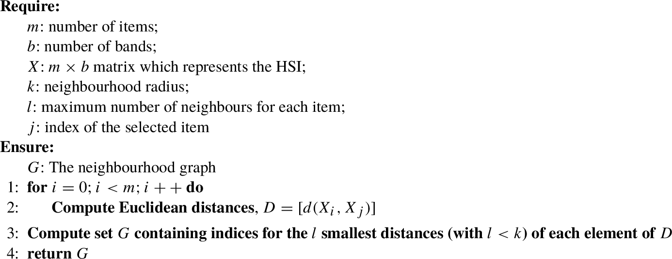
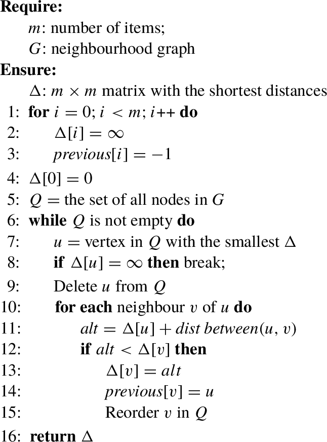
Isomap is a manifold learning algorithm which can reduce the data redundancy preserving the original geometry of it. Isomap estimates the geodesic distance between all the items, given only input-space distances. For the points which are neighbours, input-space is an accurate approximation to the geodesic distance. For the distant ones, the geodesic distance can be computed as the addition of a sequence of distances between neighbouring points. The main idea is to find the shortest paths in a graph with edges connecting neighbouring data points (Tenenbaum
et al.,
2000).
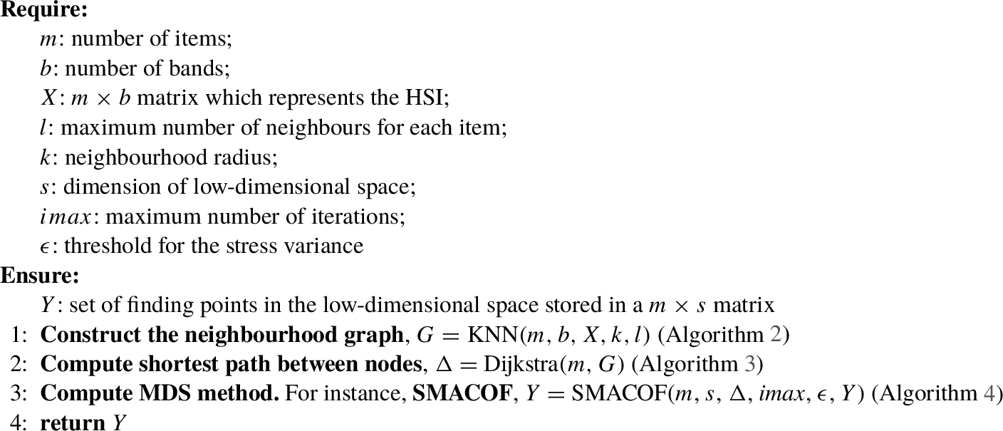
Isomap tries to build a matrix which contains all the minimum (geodesic) distances between the
m items which are contained in a data set
X (an HSI in our case), and then it reduces such matrix. In detail, the algorithm has three steps. They are shown in Algorithm
1 and described below:
Algorithm 1
Isomap(m, b, X, l, k, s, $\mathit{imax}$, ϵ)
Algorithm 2
KNN(m, b, X, k, l, j)
To evaluate the accuracy of Isomap based on SMACOF and eigen-decomposition methods for HSIs, a classification process with several classifiers – the Support Vector Machine (SVM) (Cortes and Vapnik,
1995), the KNN classifier (Altman,
1992) and the Random Forest algorithm (Breiman,
2001) – has been used.
Algorithm 3
Dijkstra(m, G)
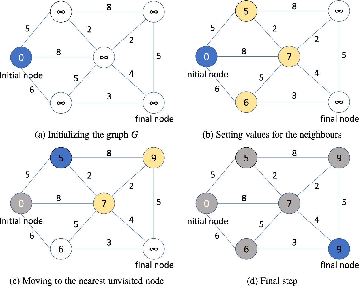
Fig. 1
Steps of the Djikstra’s algorithm.
3 SMACOF
SMACOF, as other MDS methods, is used for the analysis of similarity data on a set of items. As it has been mentioned before, SMACOF is the most accurate MDS technique (Ingram
et al.,
2009). Its objective is to find a set of points
${Y_{1}},{Y_{2}},\dots ,{Y_{m}}\equiv Y$ in a low-dimensional space
${\mathbb{R}^{s}}$,
$s<b$ (where
b is the original number of dimensions), taking into account that the distances between these points must be as similar as possible to the distance between the original points
${X_{1}},{X_{2}},\dots ,{X_{m}}\equiv X$ (Orts
et al.,
2018). The key is the stress function (Eq. (
1)). The less stress, the better results, since it measures the difference between the distances of the original points and the distances of the points in the low-dimensional space. In Eq. (
1),
δ represents the distance between points of
X, and
d does it between points of
Y.
The majorizing concept, which implies to approximate a big or complex function through another smaller or simpler, is used by SMACOF to achieve the reduction of the stress (Groenen
et al.,
1995). It consists of finding a new function iteratively. The new function will be located over the complex one, touching it at a point called
supporting point (Fig.
2). Each iteration brings the minimum of the new function closer to the minimum of the original one, that is, the stress function (Borg and Groenen,
2005; Mairal
et al.,
2014). In De Leeuw and Mair (
2011), the majorization is defined in the following steps:
-
1. To choose an initial value $y={y_{0}}$.
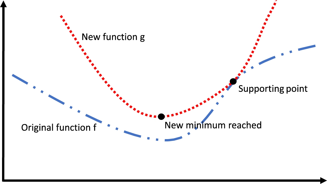
Fig. 2
Illustration of the majorization concept. The original function f is represented with a blue dashed line. The function obtained by majorization at every iteration, g, represented as a red dotted line, touches f at the supporting point. Taking into account that a new minimum of g is obtained at every iteration.
-
2. To find update ${x^{t}}$ such that $g({x^{t}},y)\leqslant g(y,y)$.
-
3. If $f(y)-f({x^{t}})\geqslant \epsilon $, then $y={x^{t}}$ and go to step 2.
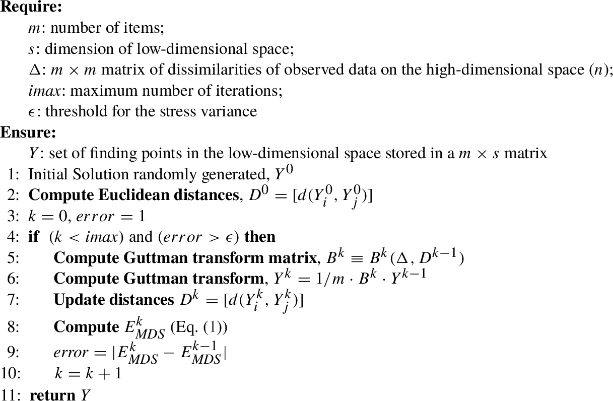
In Algorithm
4, all the steps of SMACOF are shown. In such an algorithm, the initial value
$y={y_{0}}$ mentioned in step 1 is randomly generated. It has been tested in other works in which SMACOF obtains good results beginning from solutions randomly generated (Orts
et al.,
2018). The stress value of the current mapping is measured and then compared to the stress value of the previous mapping result. Each iteration minimizes the stress value due to the generation of closer solutions to the original. If the difference between the distances is smaller than a fixed threshold value, the algorithm stops (Ekanayake
et al.,
2010), as it is mentioned in step 3. For the sake of simplicity, the details of the Guttman transform, used to update
${x^{(t)}}$, have not been explained here.
Algorithm 4
SMACOF(m, s, Δ, $imax$, ϵ)
4 Evaluation Results
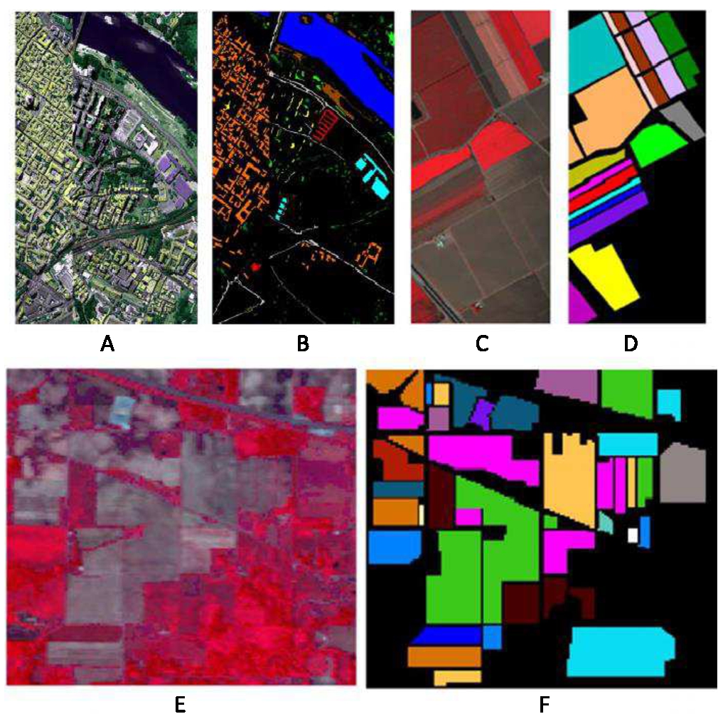
Fig. 3
HSIs tested. Pavia city centre (A) and its ground truth (B), Salinas-A (C) and its ground truth (D), and Indian Pines with its ground truth ((E) and (F) respectively).
Such an investigation methodology has been considered in this work: first, to run Isomap based on SMACOF or eigen-decomposition methods and, after that, to apply a classification process with SVM, KNN or Random Forest classifiers.
Obtained results of Isomap using SMACOF are compared with the obtained results of a recent paper where Isomap considers an eigen-decomposition process (Li
et al.,
2017) in the problem of hyperspectral images reduction. As in Li
et al. (
2017), three popular HSI images collected by the AVIRIS and ROSIS sensors have been considered to test Isomap (see Fig.
3). The considered data sets have the following characteristics:
-
• Pavia city centre (AVIRIS Salinas Valley,
2019), acquired by the ROSIS sensor. Pavia consists of
$1096\times 715$ pixels and 102 bands. For the sake of clarity, the data set is reduced to a
$150\times 150$ pixels subset. However, authors in Li
et al. (
2017) do not detail how they truncate the image in the study. In our work, random subsets of
$150\times 150$ are collected, keeping the ground truth variety.
-
• A finer spatial resolution of Salinas (AVIRIS sensor), named Salinas-A. Salinas-A consists of $86\times 83$ pixels, which are the $[samples,lines]$ $=[591-676,158-240]$ of the original Salinas data set. It contains 204 bands.
-
• The Indian Pines data set (Aviris,
2012) collected by the AVIRIS sensor. It consists of
$145\times 145$ pixels and, originally, 224 bands. However, 24 bands which contain the information about water absorption are removed in Li
et al. (
2017), so it has 200 bands in the tests.
Both Isomap versions (SMACOF and eigen-decomposition) have been implemented in Matlab and executed on a cluster composed by 64 cores of Bullx R424-E3 Intel Xeon E5 2650 with 8GB RAM. Specifically, KNN and Dijkstra procedures (Algorithms
2 and
3) have been coded using the Matlab functions
find_nn and
dijkstra, respectively. The precision of the classification process is dependent on the considered dimension of low-dimensional space (
s) on Isomap. Therefore, several dimensions
s have been taken into account to study their accuracy in the classification. Concretely, we varied the dimension of
s from 10 to 50, as it was performed in Li
et al. (
2017). The parameter
k, which describes the number of neighbours handled for each point has been set to 20.
We follow the idea described in Li
et al. (
2017) of considering several classifiers to evaluate the accuracy of both versions of Isomap for HSI classification, such as SVM and KNN classifiers. In addition, we have also considered the Random Forest algorithm. Similarly to Li
et al. (
2017), training and testing data were randomly selected from the ground truth. The
$20\% $ of the total pixels of each image were used to train, and the
$80\% $ to test. The comparative analysis has been based on the classification accuracy, which is obtained as the ratio:
correctly predicted data/
total testing data.
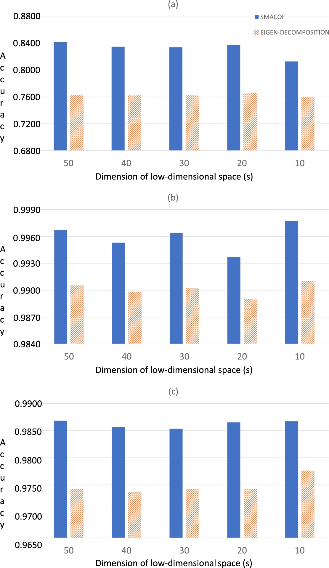
Fig. 4
Classification results (in terms of accuracy) of the three HSI data sets using SVM: (a) Indian Pines; (b) Salinas-A; (c) Pavia.
The SVM is coded using LIBSVM described in Chang and Lin (
2011) with the following parameters: “
$-t$ 2
$-c$ 100” (
$-t$ 2 sets the type of kernel function as radial basis function, and
$-c$ 100 set the cost parameter to 100). It is not necessary to set the gamma value,
$-g$ (a parameter used as input by the radial basis function), as it is automatically set to “
$-g$ $1/D$”, where
D is the dimension. The input data must be transformed following the data preprocessing described in Hsu
et al. (
2003). The results obtained using the SVM are depicted in Fig.
4.
Table 1
Classification results (in terms of accuracy) of the three HSI data sets using KNN for ${k^{\prime }}=1,3$ and 5 and test images Indian Pines, Salinas-A and Pavia.
| IMAGE |
s |
SMACOF |
EIGEN-DECOMPOSITION |
| ${k^{\prime }}$ |
| 1 |
3 |
5 |
1 |
3 |
5 |
| Indian Pines |
50 |
0.8112 |
0.7958 |
0.7943 |
0.7250 |
0.6956 |
0.6881 |
|
40 |
0.8046 |
0.7987 |
0.7912 |
0.7200 |
0.6965 |
0.6884 |
|
30 |
0.8068 |
0.7849 |
0.7814 |
0.7150 |
0.6933 |
0.6893 |
|
20 |
0.8179 |
0.8069 |
0.7845 |
0.7150 |
0.6916 |
0.6879 |
|
10 |
0.8090 |
0.7915 |
0.7877 |
0.7050 |
0.6896 |
0.6880 |
| Salinas-A |
50 |
0.9946 |
0.9931 |
0.9890 |
0.9899 |
0.9714 |
0.9658 |
|
40 |
0.9952 |
0.9913 |
0.9925 |
0.9896 |
0.9733 |
0.9654 |
|
30 |
0.9950 |
0.9935 |
0.9904 |
0.9898 |
0.9765 |
0.9645 |
|
20 |
0.9952 |
0.9917 |
0.9914 |
0.9892 |
0.9743 |
0.9699 |
|
10 |
0.9963 |
0.9890 |
0.9924 |
0.9890 |
0.9765 |
0.9687 |
| Pavia |
50 |
0.9917 |
0.9503 |
0.9488 |
0.9729 |
0.9365 |
0.9211 |
|
40 |
0.9929 |
0.9407 |
0.9463 |
0.9720 |
0.9320 |
0.9232 |
|
30 |
0.9940 |
0.9597 |
0.9525 |
0.9729 |
0.9365 |
0.9235 |
|
20 |
0.9937 |
0.9598 |
0.9526 |
0.9735 |
0.9312 |
0.9245 |
|
10 |
0.9934 |
0.9615 |
0.9576 |
0.9715 |
0.9348 |
0.9234 |
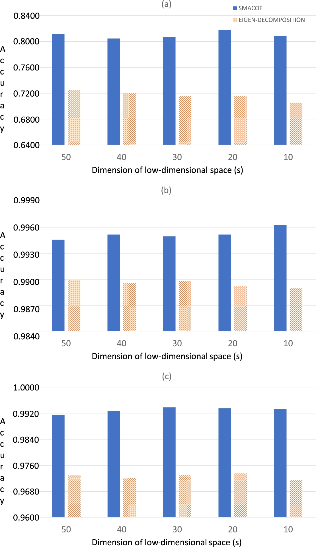
Fig. 5
Classification results (in terms of accuracy) of the three HSI data sets using 1NN: (a) Indian Pines; (b) Salinas-A; (c) Pavia.
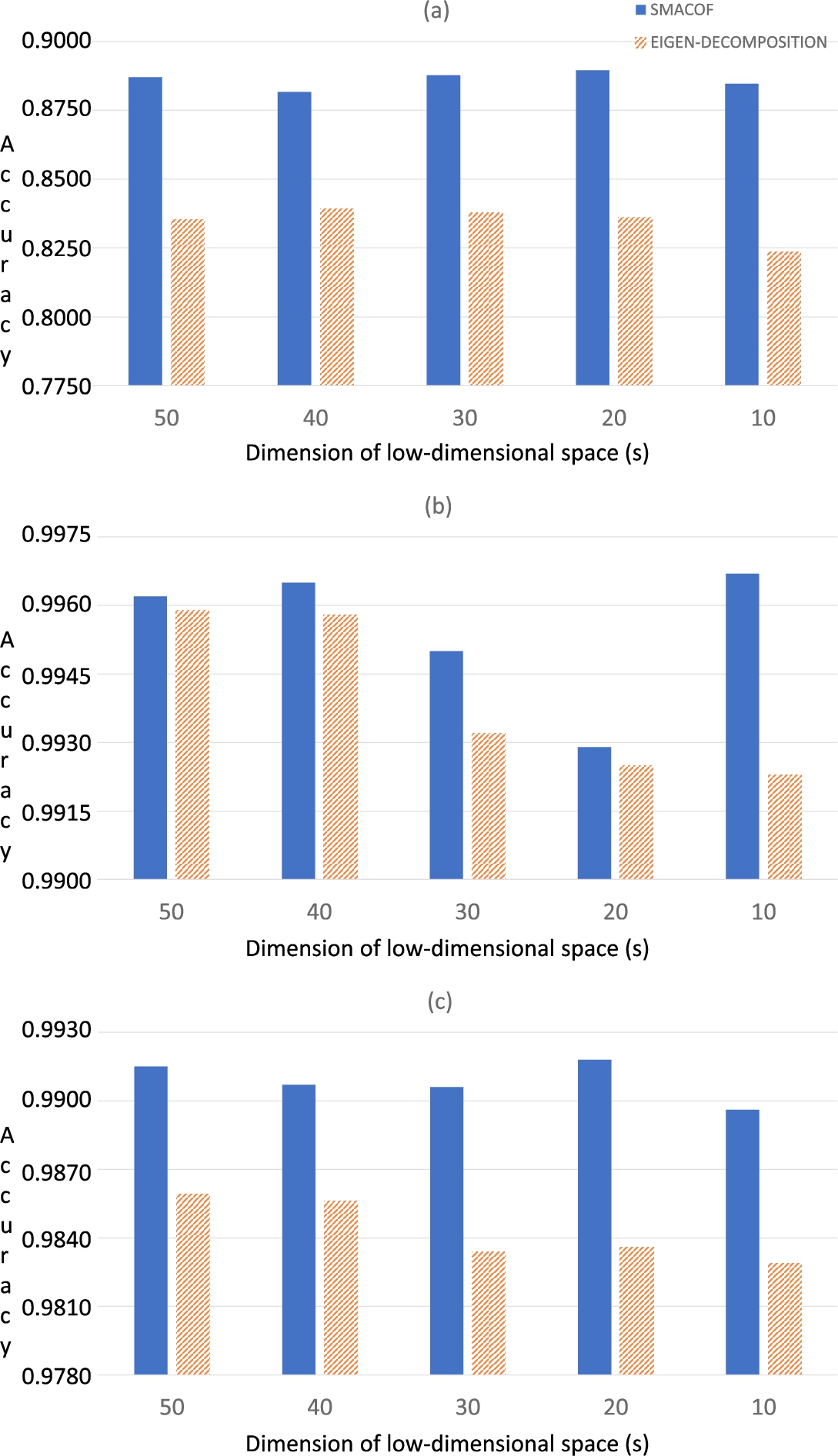
Fig. 6
Classification results (in terms of accuracy) of the three HSI data sets using Random Forest: (a) Indian Pines; (b) Salinas-A; (c) Pavia.
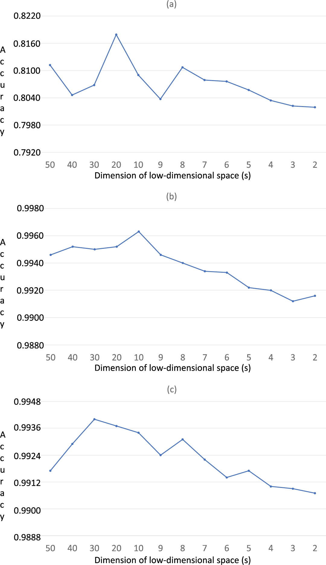
Fig. 7
Classification results (in terms of accuracy) of the three HSI data sets using 1NN for ranges from 50 to 2: (a) Indian Pines; (b) Salinas-A; (c) Pavia. Solid lines are to guide the eye.
KNN is a straightforward classification method, however, it is one of the most accurate ones (Keogh and Kasetty,
2002; Wei and Keogh,
2006). The results of the preliminary analysis of KNN are presented in Table
1 to consider the most suitable value of the number of neighbours (
${k^{\prime }}$). This table shows the accuracy of the classification considering several values of
${k^{\prime }}$ (
$1,3,5$), for every reduced image on both dimensionality reduction methods (eigen-decomposition and SMACOF). Here, the best values are marked in italic style. As it can be observed in the table, the accuracy is reduced as the value of
${k^{\prime }}$ increases and 1NN obtains the best values of accuracy in all analysed cases. Therefore, KNN with
${k^{\prime }}=1$ (1NN) will be considered hereinafter. An additional advantage of 1NN is that it does not have tuning parameters and does not require a special transformation of the data or another preprocessing (Xing
et al.,
2009). The Matlab function
fitcknn has been used to perform KNN.
Apart from the classifiers used in Li
et al. (
2017), the Random Forest algorithm has also been considered in our evaluation (Fig.
6). The Matlab function
TreeBagger has been used to perform Random Forest.
Obtained results with SVM, 1NN and Random Forest can be observed in Figs.
4,
5 and
6, respectively. The figures show the accuracy of the classification from the reduced images compared to the ground truth images, for both versions in each range from
$s=10$ to
$s=50$. Such results have shown that the use of SMACOF improves the accuracy of Isomap for the three tested classifiers. In comparison with the version based on the eigen-decomposition process, the SMACOF approach is able to achieve better accuracies which involves a more optimized classification of HSI data sets.
Once it is proven that the SMACOF approach is more accurate than the eigen-decomposition process, the global precision of Isomap with SMACOF has been tested in a more extended range of the values of
s than (Li
et al.,
2017) using 1NN (see Fig.
7). In this figure, it can be observed that the classification accuracy is quite high for all the analysed dimensionality reduction cases (from 50 to 2). However, it should be noted that the classification accuracy slightly decreases among the range from 9 to 2. Thus, we can conclude that SMACOF achieves a good accuracy even for the significant dimensionality reduction.
5 Conclusions
In this paper, our intention was to improve the accuracy of Isomap algorithm in the analysis of hyperspectral images. To achieve this, Isomap has been based on SMACOF, which is the most accurate MDS method, instead of classical scaling such as eigen-decomposition process.
The proposed version of Isomap based on SMACOF has been experimentally compared to a state-of-the-art version with an eigen-decomposition process. For that, well-known hyperspectral images taken from airbornes or satellites have been considered (Indian Pines, Salinas-A and Pavia Center). Moreover, a classification process using several classifiers (SVM, KNN and Random Forest) has been carried out to determine the accuracy of every test image with every method (SMACOF of eigen-decomposition). Obtained results have shown that the use of SMACOF improves the accuracy of Isomap in the reduction of the hyperspectral images for all studied cases.
In this work, only one criteria, the classification accuracy, is considered when reducing dimensions of the hyperspectral images. However, it should be noted that the drawbacks of Isomap and SMACOF are high consumptions of time and resources. Therefore, to decrease these aspects could be very valuable to make their application more approachable. Consequently, our current and future work is focused on the implementation of a GPU version of Isomap based on SMACOF.