1 Introduction
The human visual system is able to select the visually most important regions in its visual field. Such cognitive process allows humans to interpret complex scenes in a short and real time lapse with no need to training. Visual saliency detection is originally a problem to predict where the observer may fixate (Borji
et al.,
2015). Then, it has been extended to detect the object that attracts his gaze.
While visual saliency is highly related to human visual perception and processing, it is studied by different researches in various fields including neuro-biology (Mannan
et al.,
2009), computer vision (Borji
et al.,
2015) and cognitive psychology (Wolf,
2004). And it was used in different vision applications like object of interest detection (Donoser
et al.,
2009), object recognition (Gu
et al.,
2015), image compression (Christopoulos
et al.,
2000), image editing based on content aware (Zhang
et al.,
2009; Cheng
et al.,
2010), image retrieval (Chen
et al.,
2009), etc.
Classic segmentation problems aim to partition the input into coherent regions while salient object detection approaches aim to segment the object of interest from its surroundings.
However, detecting the salient object automatically, accurately and efficiently is very desired if we consider the high and immediate ability to grant computational resources for image processing, extract the objects features, isolate it from the background and produce the final salient object. In recent years, image saliency detection has achieved good results and the number of computational models is quite big compared to video saliency which is a quite new topic and a promising research field.
Image saliency detection covers only the spatial domain, while video saliency includes spatial and temporal information which is incorporated by the video motion information.
Actually, exploiting and using the spatial and temporal information into a video saliency framework has become a research trend in the field of video saliency detection.
The saliency of a given input is the most visible content that is able to define the human attention, called saliency map. Saliency map computation is a usually bottom-up process issued from a surprising or distinctive visual stimuli and is often assigned to brutal change in image features such as edges, boundaries, colour or gradient (Borji and Itti,
2013). The first visual saliency models were devoted to image saliency and can be grouped into two groups, namely, local and global saliency approaches. Local approaches measure rarity of a region over its neighbourhoods (Itti
et al.,
1998; Harel
et al.,
2006). In contrast, global approaches are based on the rarity and uniqueness of image regions with respect to the whole scene (Cheng
et al.,
2015; Kim
et al.,
2014). Mao
et al. (
2015) propose a saliency method inspired from the human visual system that combines local and global saliency features with high-level features (prior-knowledge, object detection) and structure saliency to highlight the object that attracts human gaze. For each saliency map, features are extracted using Adaptive-Subspace Self-Organizing Map for image retrieval. Gu
et al. (
2015) present an application of the visual saliency detection which aims to recognize the object of interest. Since the biological visual system naturally tends to focus on the region that contains the most informative object, saliency detection is used as a robust object detector. Then, features of the region that contains the object of interest are extracted using the dense Scale Invariant Feature Transform. A linear support vector machine classifier is used to define the object class. Here we only review the main papers on video saliency, for an excellent review of saliency methods in still images we refer to Borji
et al. (
2014,
2015). While saliency detection in still images has been intensively treated, spatiotemporal saliency detection is a new problem. Motion cues are a crucial foreground indicator in a video saliency detection framework; however, some background motions can blur the location of a salient object.
Only few methods adress the video saliency problem (Itti and Baldi,
2005; Zhong
et al.,
2013; Gao
et al.,
2008; Wang
et al.,
2015; Mauthner
et al.,
2015) and most of them make use of an image saliency method and simply add a motion feature as a saliency clue. Therefore, in this paper we propose a simple and effective framework that detects salient objects in videos based on spatio-temporal saliency estimation. First, for a robust saliency estimation, we use the change of contrast to indicate the main object locations. To do so, we propose a uniform contrast measure which makes use of traditional contrast features (local contrast and contrast consistency) and our novel contrast cue named spatial consistency (see Section
4.2). Spatial saliency is designed as a growing process by propagating the influence of the proposed local uniform contrast measure in the foreground-background patch assignment.
Then, for more accuracy, temporal saliency estimation is derived where we use the inter-frame temporal coherence incorporated into our motion distinctiveness feature (Section
5.1) and the intra-frame motion information presented as our four-sided motion estimator (Section
5.2). Finally, spatial and temporal saliency maps are fused into one final saliency map. The main steps of our proposed approach are introduced in Algorithm
1.
For the evaluation we use two standard benchmark data sets for video saliency, namely, the SegTrack v2 dataset proposed by Li
et al. (
2013) and Fukuchi dataset of Fukuchi
et al. (
2009).
The rest of the paper is organized as follows. In Section
2, we discuss related works. In Section
3, we present an overview of our proposed model. In Section
4, we detail our uniform contrast measure for spatial saliency estimation. In Section
5, we introduce our temporal motion estimation. Then, the final saliency map fusion is presented in Section
6. Experiments and results will be discussed in Section
7. Finally, conclusions will be provided in Section
8.
2 Related Work
Video saliency detection aims to identify the object that catches our attention from video sequences.To the best of our knowledge, the number of methods designed to address this problem is reduced. When an observer watches a video, he does not have enough time to examine the whole scene, so his gaze is always directed towards the moving object. For this reason, motion is the most important cue for detecting salient objects in videos which makes a deep exploration of the inter-frame information more crucial than ever.
Recently, different spatio-temporal saliency models have been proposed using different methods and theories such as the theory of information, control theory, the frequency domain analysis, machine learning and low rank decomposition.
Information theory based spatio-temporal saliency models use the video frames self information, the conditional entropy and the various formulations of the incremental coding length as saliency indicators.
Spatio-temporal saliency models based on the control theory represent first the video sequence with the linear systems state space model, then exploit the controllability or the observability of the linear system to discriminate the salient object and the background motion and produce the exact saliency measure (Gopalakrishnan
et al.,
2012).
Spatio-temporal saliency methods based on Frequency domain analysis generate the master saliency map using the Quatrain Fourrier Transform (QFT) phase spectrum over the feature space which contains the luminance, two chrominance components and the frame difference, and the fourrier transform amplitude spectral over the time slices at vertical and horizontal directions (Cui
et al.,
2009).
Machine learning methods use training data to build models and testing data to predict saliency map of an input video frame. Machine learning methods like probabilistic learning, support vector regression with or without Gaussian kernels are widely used (Rudoy
et al.,
2013).
The low rank decomposition methods decompose the matrix of the temporal slices into a low rank matrix that characterizes the background and a sparse matrix for salient objects (Xue
et al.,
2012).
In the literature, since there is a gap between the spatial and temporal domains, a lot of spatio-temporal duels measure the spatial and temporal saliency apart, then combine them using either a linear or a non-linear fusion schemes to provide the final spatio-temporal saliency map. Gao
et al. (
2008) proposed a spatio-temporal model issued from an image saliency model by adding a motion channel to characterize the temporal feature. Also, Mahadevan and Vasconcelos (
2010) used an image saliency model to model spatio-temporal saliency using dynamic texture. Rahtu
et al.’s (
2010) saliency model is suitable for videos and still images. It combines a conditional random field model with saliency measures formulated using local features and statistical framework. Using the centre-surround and colour orientation histograms as spatial cues and temporal gradient differences as temporal cues, Kim
et al. (
2011) proposed spatio-temporal saliency models.
In Luo and Tian (
2012), using the temporal consistency and the entropy gain, a video saliecy detection model is proposed.
Wang
et al. (
2015) proposed a spatio-temporal framework where first they determine the spatial edges of the input frame and the optical flow (used to highlight the dynamic object), then mix both spatial and temporal information to produce the exact salient object. Saliency scores are assigned using the geodesic distance. Later, the Gestalt principle of figure-ground segregation for appearance and motion cues is used by Mauthner
et al. (
2015) to predict video saliency. A spatio-temporal saliency framework using colour dissimilarity, motion difference, objectness measure, and boundary score feature is proposed by Singh
et al. (
2015) to determine each saliency score of every superpixel in the input frame.
Shanableh (
2016) proposed a video saliency method that uses intra- and inter-frame distances for the saliency maps computation. Hamel
et al. (
2016) integrated the colour information into the bottom-up saliency detection model. An effective attention model (Annum
et al.,
2018) based on texture smoothing and contrast enhancement applications is introduced for improving saliency maps in complex scenes. Bhattacharya
et al. (
2017) investigated the video decomposition model to extract the motion salient information from a video. Imamoglu
et al. (
2017) developed a multi-model saliency detection fusing salient features through both top-down and bottom-up salient cues. Given consistency of spatio-temporal saliency maps, video saliency research is still an emerging hard issue to be more investigated.
Although the aforementioned approaches process the input video in a frame by frame basis, they ignore that a prefect saliency map should be spatio-temporally coherent. It is obvious that video saliency detection is a challenging research problem to further be investigated.
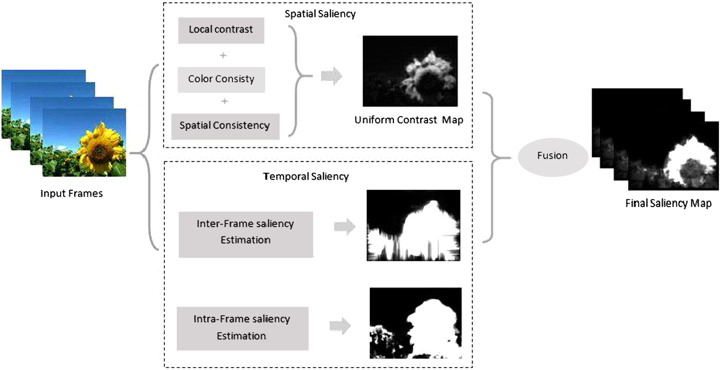
Fig. 1
Framework of the proposed method from left to right: in-out video frames, spatial and temporal saliency maps, final saliency map.
3 Proposed Model
In this section, we propose an overview of our spatio-temporal saliency framework.
Unlike state-of-the-art methods, this work produces an accurate spatio-temporal saliency maps where the object of interest is perfectly highlighted and segmented from the background. Our framework has three main steps: spatial saliency estimation, temporal saliency estimation and final spatio-temporal map generation.
Our model takes a
$n\times m\times t$ video frame
F and produces a saliency map
S, where each pixel
x has a saliency score
$S(x)=l$ and the higher this score is, the more salient this pixel is. Spatial saliency map is measured at patch level by the newly proposed uniform contrast measure which combines spatial priors with traditional contrast measure. Patches with higher uniform contrast measure are considered as salient foreground. Then, we measure the temporal saliency using our inter-frame and intra-frame motion estimators: Along a video sequence, for each frame, pixels with distinctive motion attract human gaze. Inter-frame motion estimation is performed using our motion distinctiveness measure which will highlight the object of interest that has a distinctive activity when moving from one frame to another. Intra-frame motion information is measured using our four-sided motion estimator where for each frame, we compute the magnitude gradient, then a gradient flow field is derived from the cumulative sum of the magnitude gradient through four sides of the frame. Motion information alone is insufficient to identify the object of interest in case of complex scenarios like a moving object with small optical flow or dynamic background. The use of our spatial saliency map have improved the results (see Fig.
1).
6 Saliency Maps Fusion
The final saliency map is the fusion of the static and dynamic saliency maps. The combination is performed to modify static saliency maps with the corresponding dynamic saliency value.
According to previous works on video saliency (Goferman
et al.,
2012), locations that are distant from the region of attention are less attractive than those which are around. Which means that pixels that are closer to the object of interest get higher saliency scores than further ones.
Hence, the saliency at location
$X=(x,y)$ can be defined as
where
$d(x,y)$ is the Euclidean distance between
$X=(x,y)$ and the centre
$C=({x_{c}},{y_{c}})$,
${S_{m}}(x,y)$ is the saliency values at location
$(x,y)$ and is given by
the exponential function is used to widen the contrast of the dynamic saliency weights and
$N(S(x,y))$ is a normalization operation used to normalize the values of
$S(x,y)$ to the range of
$[0,1]$. To minimize noise caused by camera motion we use a 2D Gaussian low-pass filter
${I_{k\ast k}}$,
k is the kernel value equal to 5.
All the aforementioned actions that helped to achieve better results are organized in Algorithm
1 as follows
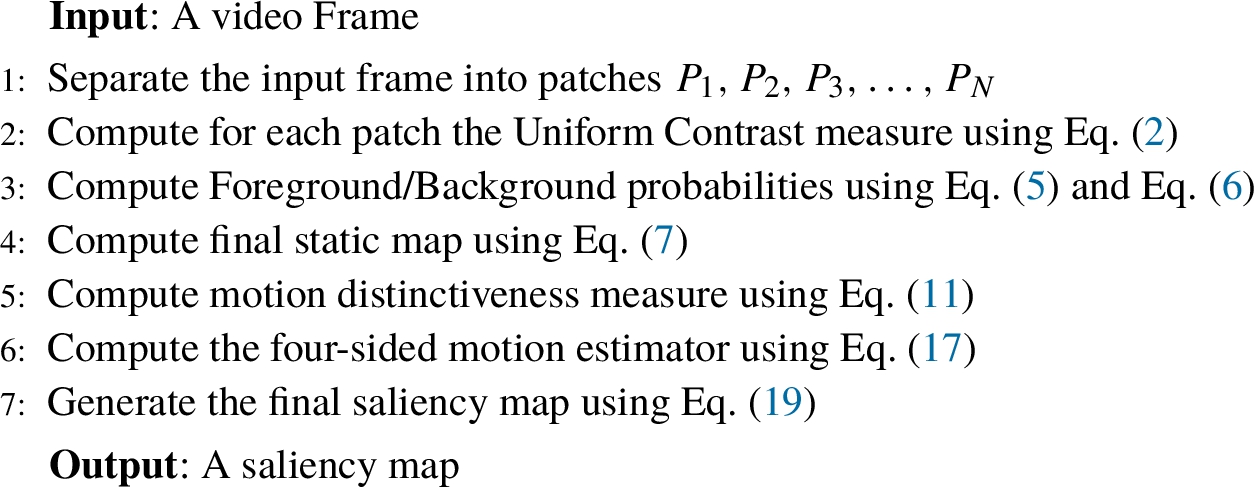
Algorithm 1
Video saliency detection.
7 Experiments
Our method detects automatically salient objects in video sequences. In this section, we compare our spatio-temporal saliency framework against state-of-the-art methods on the Segtrack v2 (Li
et al.,
2013) and Fukuchi (Fukuchi
et al.,
2009) datasets. In our proposed method, we utilize the spatial and temporal information of the input frame at pixel and frame levels to decide saliency probability of each pixel. Spatial information includes contrast cues, while temporal information makes use of motion distinctiveness and magnitude gradient flow field. The fusion of spatial and temporal saliency maps leads to a saliency map which highlights region of interest and segments salient object from the background.
7.1 Datasets
We evaluate our approach on two benchmark datasets that are used by most of the state-of-the-art video saliency methods.
Fukuchi dataset (Fukuchi
et al.,
2009) contains 10 video sequences with a total of 768 frames with one dynamic object per video. The ground truth consists of the segmented images. The dynamic objects are from different classes including horse, flower, sky-man, snow cat, snow fox, bird, etc.
SegTrack v2 dataset (Li
et al.,
2013) contains 14 sequences with a total of 1066 frames. Videos can contain more than one dynamic object. Salient objects include objects with challenging deformable shapes such as birds, a frog, cars, a soldier, etc.
7.2 Evaluation Metrics
The performance of our method is evaluated on two extensively used metrics including Precision-recall PR curves, Receiver operating characteristic ROC curves F-measure and AUC.
In the saliency detection field, precision is defined as the salient pixels that are rightly detected and is given by (
20)
Recall is the percentage of the detected salient pixels and is given by (
21)
where
$S(x,y)$ is the saliency degree of pixel
$p(x,y)$ in the obtained saliency map, and
$G(x,y)$ is the saliency degree of the pixel
$p(x,y)$ in the ground truth. The precision-recall curves are build by binarizing the saliency maps of each method using a fixed threshold. They are computed by varying the threshold from 0 to 255.
PR curves offer a reliable comparison of how good the saliency maps are and how well they highlight salient regions in a video frame. The
F-measure is defined as:
where we use
${\beta ^{2}}=0.3$ following (Li
et al.,
2014).
The ROC curve plots the true positive rate against the false positive rate. A perfect approach has a 0 value for the false positive rate and 100 per cent value for the true positive rate which indicates that predictions are identical to the ground truth.
While ROC curves evaluate the performance of a model as two-dimensional representation, the AUC elaborates this information into a single measure. As the name signifies, it is calculated as the area under the ROC curve. A perfect model will score an AUC of 1, while random prediction will score an AUC of around 0.5.
7.3 Implementation
The implementation of the proposed Algorithm
1 can be divided into two main steps, namely, static map generation and dynamic map generation. To generate the static map, we divide the input video into frames, where each frame is treated as an independent image. Then each video frame is divided into non-overlapping square patches (patch width equal to 2). For each patch, the second step of Algorithm
1 is computed using local contrast, contrast consistency and spatial consistency features. Local contrast aims to compute the contrast change between a pair of patches, which highlight the object’s boundaries. Contrast consistency measures the contrast weight between two patches regarding the neighbouring ones which will emphasize the whole object. Local contrast and contrast consistency will emphasize the object and its border. Spatial consistency measure is based on the assumption that distant patches highly belong to different objects. Unified contrast measure will be used to label each patch as a foreground or background patches where foreground patches belong to the salient object and background patches belong to background which are then used to compute foreground/background probabilities. The final static map is then computed (Algorithm
1, fourth step).
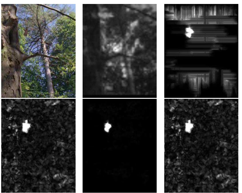
Fig. 3
Spatio-temporal saliency map. From left to right: Input frame, spatial map, four-sided motion map, motion distinctiveness map, saliency map and ground-truth.
The second part of our proposed method starts at step 5 of the proposed Algorithm
1 which consists on computing the temporal saliency degree of each frame. To do so, two saliency measures are proposed: the first is the motion distinctiveness measure which is proposed under the assumption that suspicious motion attracts attention (see Section
5.1), and the four-sided motion estimator which is used to compute motion consistency between each pair of frames (see Section
5.2). Temporal saliency measures and static saliency map are fused together to generate the final saliency map.
Figure
3 details the exact resultant map at each step. First the spatial map is generated, we notice that the colour of the falling bird is quite similar to the colour of the trees limbs which enables the uniform contrast measure to detect the salient object. So, we use the four-sided motion estimator and motion distinctiveness measure (see Section
5.2 and Section
5.1) to extract the salient object (falling bird). We notice that in challenging cases where the contrast and spatial consistencies can not segment the object of interest from the background, temporal cues are essential to highlight the salient object.
7.4 Results
We compare our video saliency approach to seven state-of-the-art methods, namely, CBS (Jiang
et al.,
2011), GB (Harel
et al.,
2006), GVS (Wang
et al.,
2015), ITTI (Itti and Baldi,
2005), RR (Mancas
et al.,
2011) and RT (Rahtu
et al.,
2010).
On both Segtrack v2 and Fukuchi datasets we clearly outperform the other methods in terms of F-measure and AUC. The precision-recall curves in Fig.
4 provide similar conclusions where our method obtains best results compared to the state-of-the-art methods for most recall values.
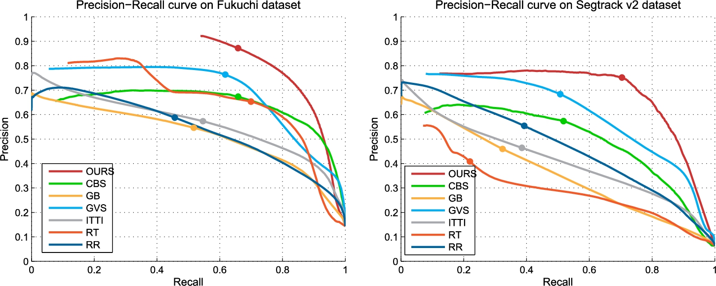
Fig. 4
PR curves on Fukuchi and Segtrack v2 datasets.
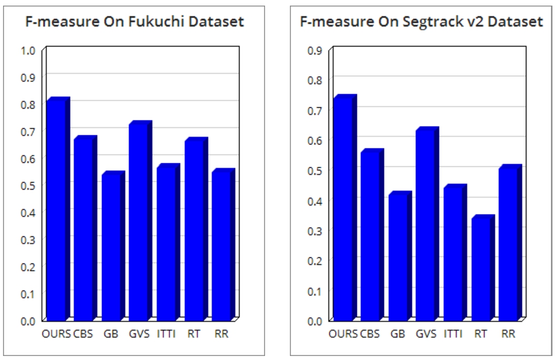
Fig. 5
F-measure values on Fukuchi and Segtrack v2 datasets.
Recall values of
RR (Mancas
et al.,
2011) and
GVS (Wang
et al.,
2015) are very small when we vary the threshold to 255 and even decrease it to 0 in case of
ITTI (Itti and Baldi,
2005),
RT (Rahtu
et al.,
2010) and
GB (Harel
et al.,
2006) since the output saliency maps do not respond to the salient object detection. For the Segtrack v2 and Fukuchi datasets, the minimum value of recall does not decrease to zero which means that in the worst case and with the most complex background, our method detects the region of interest with good response values. Moreover, our saliency method attains the best precision rate, which denotes that our detected saliency maps are more responsive to regions of interest. The obtained F-score results are 0.739 on Segtrack v2, and 0.829 on Fukuchi (see Fig.
5).
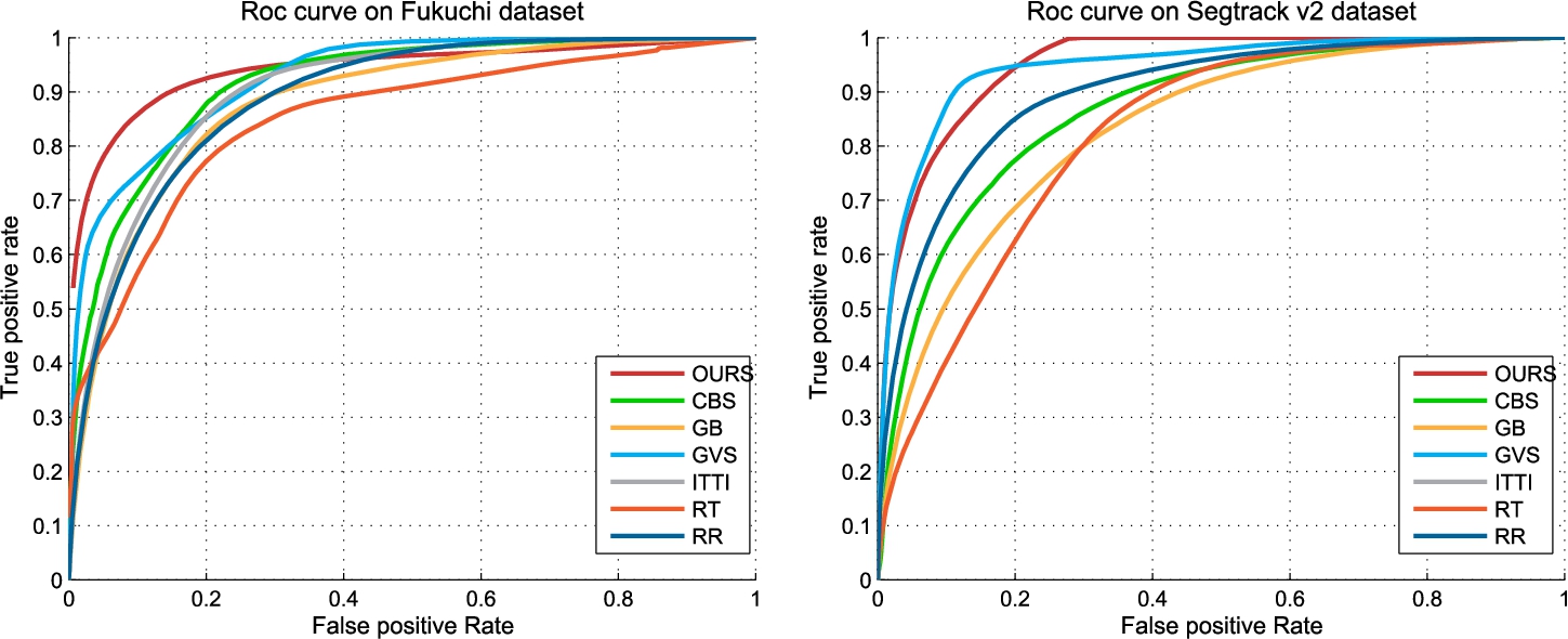
Fig. 6
ROC curves on Fukuchi and Segtrack v2 dataset.
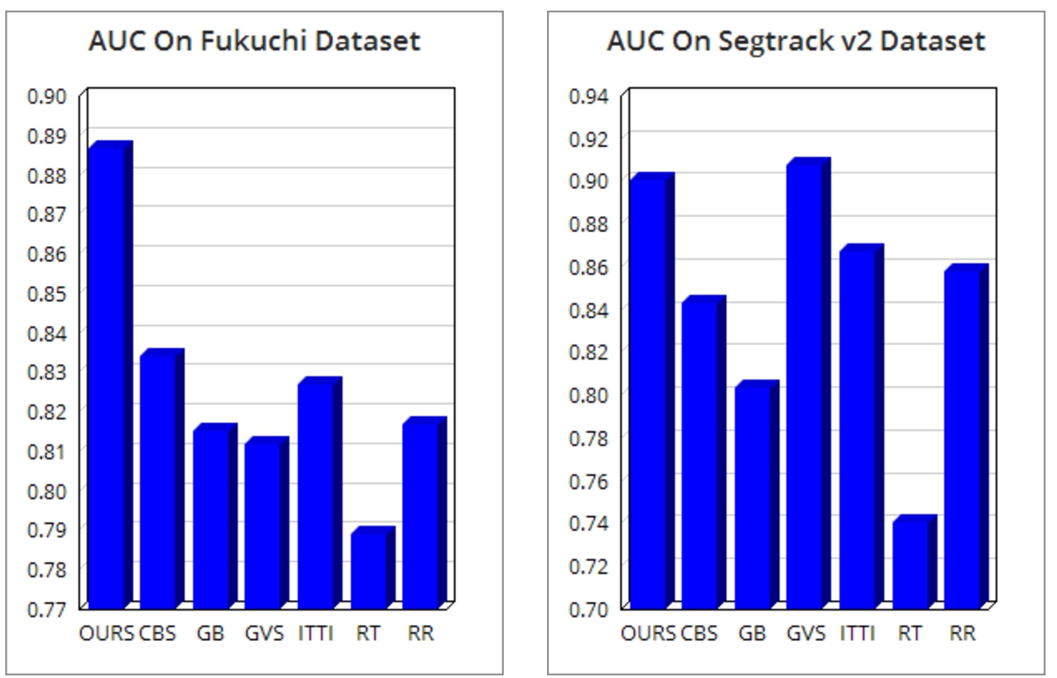
Fig. 7
AUC values on Fukuchi and Segtrack v2 dataset.
ROC curves are presented in Fig.
6. For low false positive rate our method obtains much higher true positive rates. The area under ROC curves are also reported in Fig.
7 where we reach best values on both datasets.
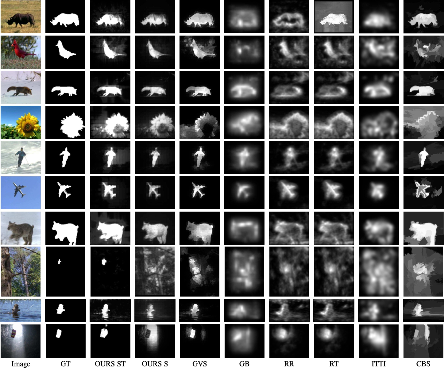
Fig. 8
Visual comparison of saliency maps generated from 6 different methods, including our method using the spatio-temporal features, our method using only spatial features, GVS (Wang
et al.,
2015), GB (Harel
et al.,
2006), RR (Mancas
et al.,
2011), RT (Rahtu
et al.,
2010), ITTI (Itti and Baldi,
2005) and CBS (Jiang
et al.,
2011)
We added qualitative comparison on different challenging cases in Fig.
8 and in each situation, our method outperforms other methods. Saliency maps provided by
GB (Harel
et al.,
2006) and
ITTI (Itti and Baldi,
2005) and do not show the exact location of the salient object because of lack of motion information, especially with complex backgrounds.
RT (Rahtu
et al.,
2010) is quite good, the salient object is correctly detected but the background gets high saliency probability. While optical flow is one of the most used techniques to detect moving objects, it can not be a good saliency estimator. The performance of video saliency detector
RR (Mancas
et al.,
2011) based on optical flow, assign low saliency probability to static pixels which belong to salient object (see third and sixth rows). In most cases,
CBS (Jiang
et al.,
2011) and
GVS (Wang
et al.,
2015) are able to locate the salient object even in complex situations where foreground-background colours are similar (see eighth rows) since their motion information is very informative. Results of a moving object with higher speed and a static camera are shown in the third row, and produce a good saliency map. In case of an object with high speed and a moving camera (fifth and sixth rows), our proposed motion feature highlights only the moving object. Based on the aforementioned analysis, two main conclusions can be drawn. First, to detect a salient object in videos, it is essential to examine motion information. Second, developing a method that depends only on motion information is not an excellent idea. Combining spatial and temporal information into a video saliency framework leads to the best results.
We performed an extra test, where we use only uniform contrast measure to detect saliency (see second column of Fig.
8). We notice that when there is a change of contrast between the background and the object, the salient object can be correctly detected and the role of motion feature is to set up the regions of the object that made a remarkable movement (e.g. the flower and the wolf). In case of colour similarity between the salient object and the background, the use of static information will fail to point out the object of interest, and the use of motion features will accomplish the mission (e.g the falling bird and the parachute). In this work, we use an inter-frame and intra-frame motion estimation to reinforce temporal saliency detection. Inter-frame motion estimation is performed using our motion distinctiveness measure which will highlight the object of interest that has a distinctive activity when moving from one frame to another. Intra-frame motion information is measured using our four-sided motion estimator where for each frame, we compute the magnitude gradient, then a gradient flow field is derived from the cumulative sum of the magnitude gradient through four sides of the frame. Our motion features are able to face challenging situations like slow motion, noise caused by optical flow.